Prediction of Target Detection Probability Based on Air-to-Air Long-Range Scenarios in Anomalous Atmospheric Environments - MDPI

Page created by Jane Jensen
 
CONTINUE READING
Prediction of Target Detection Probability Based on Air-to-Air Long-Range Scenarios in Anomalous Atmospheric Environments - MDPI
remote sensing
Communication
Prediction of Target Detection Probability Based on Air-to-Air
Long-Range Scenarios in Anomalous Atmospheric Environments
Tae-Heung Lim and Hosung Choo *

                                          The Department of Electronic and Electrical Engineering, Hongik University, Seoul 04066, Korea;
                                          qpzm0105@mail.hongik.ac.kr
                                          * Correspondence: hschoo@hongik.ac.kr

                                          Abstract: We investigate a target detection probability (TDP) using path loss of an airborne radar
                                          based on air-to-air scenarios in anomalous atmospheric and weather environments. In the process
                                          of calculating the TDP, it is necessary to obtain the overall path loss including the anomalous
                                          atmospheric environment, gas attenuation, rainfall attenuation, and beam scanning loss. The path
                                          loss including the quad-linear refractivity model and other radar input parameters is simulated
                                          using the Advanced Refractive Effects Prediction System (AREPS) software along the range and
                                          the altitude. For the gas and rainfall attenuations, ITU-R models are used to consider the weather
                                          environment. In addition, the radar beam scan loss and a radar cross section (RCS) of the target are
                                          considered to estimate the TDP of the airborne long-range radar. The TDP performance is examined
                                          by employing the threshold evaluations of the total path loss derived from the detectability factor and
                                          the free-space radar range equation. Finally, the TDPs are obtained by assuming various air-to-air
                                scenarios for the airborne radar in anomalous atmospheric and weather environments.
         

Citation: Lim, T.-H.; Choo, H.            Keywords: air-to-air propagation; abnormal atmospheric environment; weather environment; target
Prediction of Target Detection            detection probability (TDP); long-range radar
Probability Based on Air-to-Air
Long-Range Scenarios in Anomalous
Atmospheric Environments. Remote
Sens. 2021, 13, 3943. https://doi.org/    1. Introduction
10.3390/rs13193943
                                                With the dramatic advances of radar system design technologies, the use of long-range
                                          airborne radar systems, such as synthetic aperture radars (SARs), airborne early warning
Academic Editors: Isaac Ramos and
                                          (AEW) radars, and active electronically scanned array (AESA) radars, has been growing
Adriano Camps
                                          extensively [1–6]. Such airborne radar systems essentially require high-performance spec-
                                          ifications for each component to increase the detection probability of long-range targets.
Received: 26 August 2021
Accepted: 28 September 2021
                                          However, the TDP can often be degraded by environmental or external factors including
Published: 2 October 2021
                                          noises, clutter, atmospheric gas attenuation, multipath interference, atmospheric refraction,
                                          and rainfall attenuation. To be specific, an anomalous atmospheric refractive index includ-
Publisher’s Note: MDPI stays neutral
                                          ing an unusual or abnormal distributions of temperature and relative humidity along the
with regard to jurisdictional claims in
                                          altitude can cause the refraction of the electromagnetic (EM) wave propagation different
published maps and institutional affil-   from that in normal conditions, i.e., sub-refraction, super-refraction, and ducting [7–9].
iations.                                  These wave refractions can mislead the accuracy of target position predictions, and in the
                                          worst case, long-range targets can be missed under anomalous atmospheric conditions.
                                          Therefore, it is important to model the detailed atmospheric refractive index in order
                                          for the precise predictions of the propagation path loss and propagation factor. Many
Copyright: © 2021 by the authors.
                                          studies have been conducted to model the refractive index under anomalous atmospheric
Licensee MDPI, Basel, Switzerland.
                                          conditions through the radar signal measurement [10–12], global positioning system tro-
This article is an open access article
                                          pospheric delay observation [13], and statistical analysis of the stored meteorological
distributed under the terms and           observatory data [14,15]. In addition, various studies have been conducted to analyze the
conditions of the Creative Commons        wave propagation characteristics in consideration of low-altitude actual atmospheric data
Attribution (CC BY) license (https://     in ground-to-ground and ground-to-air scenarios. For example, the real atmospheric data
creativecommons.org/licenses/by/          of specific coastal areas in the UK [16], United States [17], Greece [18], China [19], and
4.0/).                                    Korea [20] are used to calculate the long-range path loss using the propagation models,

Remote Sens. 2021, 13, 3943. https://doi.org/10.3390/rs13193943                                       https://www.mdpi.com/journal/remotesensing
Prediction of Target Detection Probability Based on Air-to-Air Long-Range Scenarios in Anomalous Atmospheric Environments - MDPI
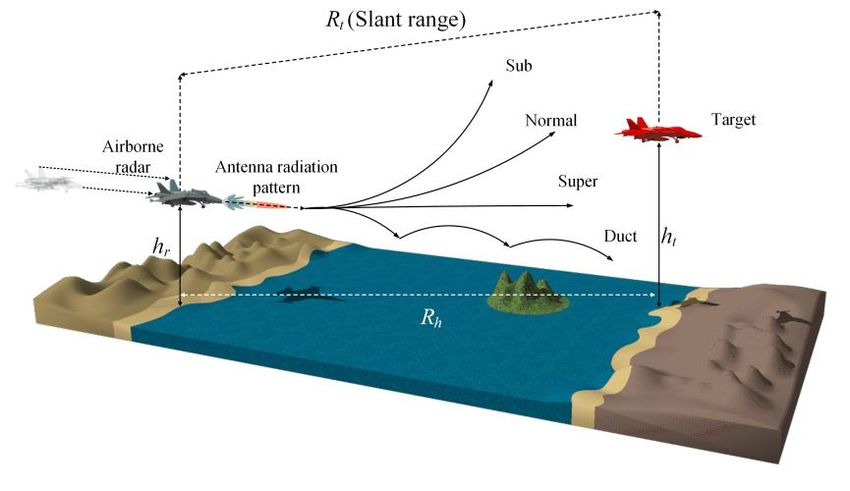
Remote Sens. 2021, 13, 3943                                                                                           2 of 14

                              i.e., the parabolic equation model, ray optics model, waveguide mode model, and hybrid
                              model [21–25]. These aforementioned studies have demonstrated the high accuracy of
                              the path loss estimation in low-altitude situations. However, their path loss calculation
                              processes need more in-depth consideration of the weather or atmospheric environment
                              to observe the air-to-air airborne radar propagation characteristics at a high altitude over
                              5 km.
                                     In this paper, we propose a TDP calculation process for the airborne long-range radar
                              based on air-to-air scenarios in anomalous atmospheric environments. In the proposed
                              process, it is necessary to obtain the overall path loss including the anomalous atmospheric
                              environment, gas attenuation, rainfall attenuation, and beam scanning loss. To observe
                              the airborne radar path loss in an anomalous atmospheric environment, the refractive
                              index as a function of altitude is modeled using four linear lines to represent various wave
                              refractions. Then, the path loss, including the refractivity model along the range and the
                              altitude, is simulated using the AREPS software [26], which is a commercial software based
                              on a hybrid model with a parabolic equation model and raytracing model. In this AREPS
                              simulation, the radar antenna beam pattern and the digital terrain elevation data (DTED)
                              are also employed as input parameters to accurately predict the airborne radar propagation.
                              The 32 × 32 airborne radar array antenna with a triangular array configuration is used
                              to calculate the radiation pattern, and the DTED of the southwest region in South Korea
                              from the National Geographic Information Institute is employed. For gas and rainfall
                              attenuations, ITU-R models are used to consider the weather environment in accordance
                              with the water vapor pressure and precipitation. In addition, the radar beam scan loss and
                              RCS of targets are considered to estimate the TDP of the airborne long-range radar. Finally,
                              the TDPs are examined by assuming various air-to-air scenarios in anomalous atmospheric
                              and weather environments.

                              2. TDP Simulation Process
                              2.1. Anomalous Atmospheric Refractivity and Measurement
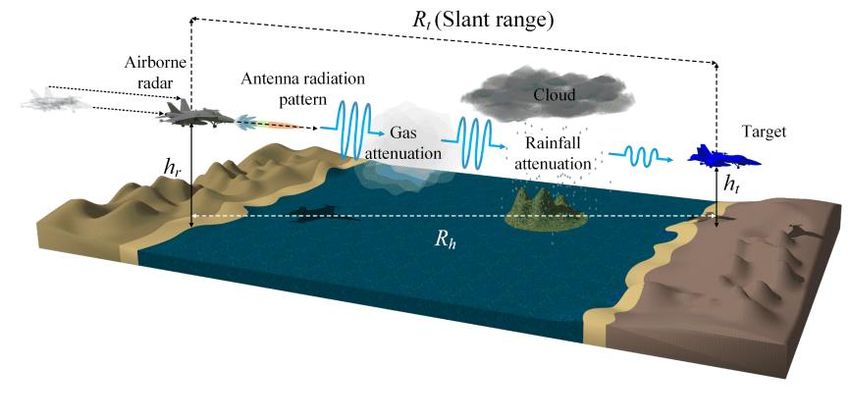
                                   Figure 1 shows a conceptual figure of the air-to-air airborne radar wave propagation
                              in accordance with an anomalous atmospheric environment. The gray and red aircrafts
                              indicate an airborne radar and a target, which are located at heights of hr and ht , having a
                              distance of Rt (slant range) and a horizontal range of Rh . The target is placed under various
                              atmospheric conditions according to the wave refraction. To observe the wave refraction of
                              the airborne radar, the refractive index needs be calculated using the measured atmospheric
                              data such as temperature, air pressure, and relative humidity based on Equations (1)–(3),
                              which are usually obtained by employing a rawinsonde or a GPS sonde [27–29].

                                                                               77.6p es 3.73 · 105
                                                        N = (n − 1)106 =            +                                    (1)
                                                                                 T         T2
                                                                             rh6.105e x
                                                                      es =                                               (2)
                                                                                100
                                                                     T − 273.2
                                                                                                
                                                                                             T
                                                         x = 25.22             − 5.31 ln                                 (3)
                                                                        T                  273.2
                              where p, T, rh indicate air pressure in hPa, temperature in K, and relative humidity in
                              %. Then, the modified refractive index M at a height of h needs to be calculated using
                              Equation (4) [30]. An example for a calculation of the modified refractive index M based on
                              the measured data from Heuksando Meteorological Observatory [31] is listed in Table 1.

                                                                     M = N + 0.157h.                                     (4)
Prediction of Target Detection Probability Based on Air-to-Air Long-Range Scenarios in Anomalous Atmospheric Environments - MDPI
Remote Sens. 2021, 13, x FOR PEER REVIEW                                                                                                            3 of 14

         Remote Sens. 2021, 13, 3943                                                                                                                            3 of 14

                                                                                        M  N  0.157h.                                               (4)

                                             Figure 1. Airborne radar wave propagation for TDP in accordance with anomalous atmospheric en-
                                   Figure 1. Airborne radar wave propagation for TDP in accordance with anomalous atmospheric
                                             vironment.
                                   environment.

                                             Table 1. Modified
                                   Table 1. Modified  refractive refractive index
                                                                  index based     based on measured
                                                                               on measured           data (32017).
                                                                                           data (3 January   January 2017).

                                                    Air PressureAir Pressure (hPa)              Relative Humidity  ◦              Relative
                                                                                                                                   Refractivity (M-      Refractivity
                                    Height (m)Height (m)                Temperature (°C) Temperature ( C)                    Humidity (%)                 (M-Unit)
                                                         (hPa)                                              (%)                           Unit)
                                        80             80 1015                1015 6                      6 87                       87 333.7                333.7
                                                     752.2                   934.8                       4.5                         9.6                     383.3
                                       752.2             934.8                    4.5                        9.6                          383.3
                                                    1477.2                   855.1                       4.7                        14.5                     476.7
                                      1477.2             855.1
                                                    2229.8                   779.64.7                    2.914.5                    10.1 476.7               572.9
                                      2229.8             779.6
                                                    2999.6                   708.22.9                   –2.710.1                    10.6 572.9               676.9
                                      2999.6        3793.1
                                                         708.2               640.3
                                                                                 –2.7                   –7.910.6                    10.3  676.9              784.7
                                      3793.1             640.3                   –7.9                       10.3                          784.7
                                                    The gradient of the modified refractive index along the height ∇M can determine
                                        The four
                                              gradient
                                                    common of the   modified
                                                                  wave           refractive
                                                                         propagation          index along
                                                                                          refractions:    normal the height
                                                                                                                       refraction  M(79       ∇M ≤ 157), super-
                                                                                                                                        can< determine
                                   four common
                                             refraction       < ∇M ≤ 79),refractions:
                                                     wave(0propagation          sub-refraction normal       ∇M), and(79
                                                                                                 (157
Prediction of Target Detection Probability Based on Air-to-Air Long-Range Scenarios in Anomalous Atmospheric Environments - MDPI
Remote Sens. 2021, 13, 3943                                                                                                                              4 of 14

                                      calculating the array factor of a 32 × 32 airborne radar array antenna using a triangular
                                      array configuration [31]. The array distances along the x- and y-axes are 0.475λ and 0.538λ
                                      at 10 GHz. This radiation pattern has a half-power beamwidth of 2.85◦ and a side lobe level
                                      of 13.5 dB. The DTED of the southwest region in South Korea are obtained from the Korean
                                      National Geographic Information Institute [33]. Then, the path loss computed using the
                                      AREPS software can be defined as LAREPS (m1 , m2 , m3 , m4 , h1 , h2 , h3 , Rh , hr , ht ) considering
                                      the anomalous environment. For example, with specific input parameters (m1 = m2 = m3
                                      = m4 = 85, h1 = h2 = h3 = 15 km, Rh = 150 km, hr = 11 km, and ht = 5 km), we can obtain
Remote Sens. 2021, 13, x FOR PEER REVIEW
                                      the path loss LAREPS of 163.5 dB in the elevated ducting of the anomalous atmospheric          4 of 14
                                      environment.

                                                               (a)                                                                            (b)
                                  Figure 2. Modified refractivity according to height: (a) the quad-linear refractivity model; (b) com-
                                     Figure 2. Modified refractivity according to height: (a) the quad-linear refractivity model; (b) com-
                                  parisons between the actual refractivity data and the quad-linear models.
                                     parisons between the actual refractivity data and the quad-linear models.

                                        The
                                     2.2.    dottedEnvironment
                                          Weather      and dash-dotted
                                                                    Modelslines denote those on September 26, 2017. To model the
                                  actual refractive    index on  July  25, 2017, theof
                                           Figure 3 illustrates the attenuation               slopes
                                                                                                 the waveof m1propagation
                                                                                                                , m2, m3, and m      by4 are
                                                                                                                                         the 125.9,  875, −25.6,
                                                                                                                                               atmospheric   gases
                                  andand142. The heights
                                          rainfall.          of h1, h2conditions
                                                      Such weather     , and h3 arecan        sethave
                                                                                                   to bea 6223,
                                                                                                              serious    6239,
                                                                                                                            impactand on6399
                                                                                                                                           them.   Theloss,
                                                                                                                                                 path   second
                                                                                                                                                            which
                                  refractivity
                                     is directlydata   on September
                                                   related to the TDP26,       2017, are also
                                                                          performance             of modeled
                                                                                                      the airborne     using    the quad-linear
                                                                                                                             radar.   Hence, it is model     (m1 to
                                                                                                                                                     necessary
                                  = 140.8,  m   = −18.9, m   = 142.6,  m    =   136.7,     h   =  5680    m,   h   =    5786
                                     have the detailed attenuation models to increase the accuracy of the TDP estimation in
                                              2            3              4                  1                   2             m,   and   h 3 = 6459  m). These
                                  quad-linear     refractivity
                                     the air-to-air   airbornemodels
                                                                radar wave have propagation.
                                                                                     2001 data points      The along
                                                                                                                   atmosphericthe altitude,     which are can
                                                                                                                                        gas attenuation     em- be
                                  ployed   as  input   parameters   for    the     AREPS
                                     modeled based on ITU-R P.676-12 as follows [34]:           software       to  obtain       the  path    loss according   to
                                  the range and altitude. Furthermore, the other input parameters of the antenna beam pat-
                                                                                                   00                00
                                  tern and DTED are also applied       γgto  =the  0.1820
                                                                                       AREPS f NOx     ( f ) + NWat
                                                                                                    simulation               f)
                                                                                                                         to(precisely     estimate the air-to-(5)
                                  air wave propagation path loss. The                antenna       beam      pattern        is derived     by calculating the
                                  array factor of a 32 × 32 airborne N
                                                                                00
                                                                                          = ∑antenna
                                                                               Ox ( f )array
                                                                             radar                 Si,ox Fi +using
                                                                                                                      00
                                                                                                                  ND ( f a) triangular array configura-(6)
                                                                                                i
                                  tion [31]. The array distances along the x- and y-axes are 0.475 and 0.538at 10 GHz. This
                                                                                    NWat ( f ) = ∑
                                                                                      00
                                  radiation pattern has a half-power beamwidth                        of S2.85°
                                                                                                            i,Wat F  and
                                                                                                                       i     a side lobe level of 13.5 dB.(7)
                                                                                                       i
                                  The DTED of the southwest region in South Korea are obtained from the Korean National
                                                                                                  3
                                  Geographic Information Institute [33].                 Then, the        path loss computed                using the AREPS
                                                                                                                               
                                                                                    −7 300                                   300
                                  software can be defined asi,oxS      =
                                                                   LAREPS (ma  10                     exp     a      1   −
                                                                              1 1, m2, m3, m4, h1, h2, 2h3, Rh, hr, ht) considering   P              the anom-(8)
                                                                                             T                                T
                                  alous environment. For example, with specific                   input      parameters          (m
                                                                                                                                     1 = m2 = m3 = m4 = 85, h1
                                                                                                   3.5         
                                  = h2 = h3 = 15 km, Rh = 150Skm, h=    r = 11 km,         300                                 300
                                                                 i,Wat      b1 10−1 and ht = 5exp          km),b we1 can
                                                                                                                   2       − obtaine the path loss LAREPS(9)
                                  of 163.5 dB in the elevated ducting of the anomalous        T               atmospheric        T environment.
                                                                                    L g = γg Rt                                           (10)
                                  2.2. Weather Environment Models
                                     where γg is the specific gas attenuation in dB/km, and f is the frequency in GHz. N00 Ox
                                        Figure 3 illustrates the attenuation of the wave propagation by the atmospheric gases
                                     and N00 Wat are the imaginary parts of complex refractivities in terms of oxygen and water
                                  and rainfall. Such weather conditions can have a serious impact on the path loss, which00is
                                     vapor. Si,Ox and Si,Wat are the strengths of the ith oxygen and water vapor lines, and N D (f )
                                  directly related to the TDP performance of the airborne radar. Hence, it is necessary to
                                     is the dry continuum. P and e are dry air and water vapor partial pressures in hPa, and T is
                                  have
                                     thethe  detailed
                                          absolute    attenuationinmodels
                                                    temperature     K. Fi is to
                                                                              theincrease
                                                                                   oxygenthe   accuracy
                                                                                           or water     of the
                                                                                                     vapor  lineTDP estimation
                                                                                                                 shape. a1 , a2 , b1in  the b
                                                                                                                                     , and    2
                                  air-to-air airborne  radar  wave  propagation.      The atmospheric   gas attenuation  can   be   mod-
                                     are the line strength coefficients. The detailed coefficient values are listed in tables in [34].
                                  eled  based
                                     Thus,  theon
                                                gasITU-R  P.676-12
                                                     attenuation    as follows
                                                                  according    to[34]:
                                                                                   the range Rt can be defined as Lg in Equation (7).
                                                                                              
                                                                              g  0.1820 f N Ox  f   N Wat
                                                                                                      ''                        ''
                                                                                                                                      f                (5)
                                                                                   ''
                                                                                 N Ox    f   S         i , ox
                                                                                                                    Fi  N D
                                                                                                                           ''
                                                                                                                                     f                  (6)
                                                                                                  i
Prediction of Target Detection Probability Based on Air-to-Air Long-Range Scenarios in Anomalous Atmospheric Environments - MDPI
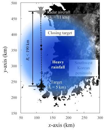
where γg is the specific gas attenuation in dB/km, and f is the frequency in GHz. N″Ox and
                         N″Wat are the imaginary parts of complex refractivities in terms of oxygen and water vapor.
                         Si,Ox and Si,Wat are the strengths of the ith oxygen and water vapor lines, and N″D(f) is the
                         dry continuum. P and e are dry air and water vapor partial pressures in hPa, and T is the
                         absolute temperature in K. Fi is the oxygen or water vapor line shape. a1, a2, b1, and b2 are
Remote Sens. 2021, 13, 3943                                                                                                                    5 of 14
                         the line strength coefficients. The detailed coefficient values are listed in tables in [34].
                         Thus, the gas attenuation according to the range Rt can be defined as Lg in equation (7).

                                Figure 3. Wave propagation attenuation by atmospheric gases and rainfall.
                     Figure 3. Wave propagation attenuation by atmospheric gases and rainfall.
                                     In addition, the rainfall attenuation can be modeled based on ITU-R P.530-17, P.837-7,
                                and P.838-3
                          In addition,       as follows
                                       the rainfall     [35–37]:can be modeled based on ITU-R P.530-17, P.837-
                                                    attenuation
                     7, and P.838-3 as follows [35–37]:                    γr = κρα                                    (11)

                                                                              r           1                          (11)
                                                        r=                                                                                       (12)
                                                             0.477R0.633
                                                                   t     ρ0.0173α
                                                                          0.01    f 0.123    − 10.579(1 − exp[−0.024Rt ])
                                                                                       1
                                                   r                  0.0173 0.123
                                                        0.477 Rt0.633 0.01   f       10.579   rRt0.024Rt 
                                                                                           de f f1 =exp                           (12)          (13)
                                                                                      Lr = γr de f f                                               (14)
                                                                             deff  rRt                                               (13)
                                 where γr is the specific rainfall attenuation in dB/km, and ρ is the rainfall precipitation
                                 in mm/h. α and κ are the rainfall                r deff
                                                                           Lr attenuation          parameters that depend on(14)      the frequency,
                                 polarization state, and angle of the signal path to the target. deff is the effective propagation
                     where γr is the specific rainfall attenuation in dB/km, and  is the rainfall precipitation in
                                 distance considering the target range Rt multiplied by the scale factor of r. The rainfall
                     mm/hr. α and κ are the rainfall attenuation parameters that depend on the frequency, po-
                                 attenuation in terms of the range can be defined as Lr in Equation (11).
                     larization state, and angle of the signal path to the target. deff is the effective propagation
                                        In general, the precipitation is measured using rain gauge, weather radar, and satel-
                     distance considering
                                 lite, and the  themeasured
                                                    target range      Rt multiplied
                                                                 weather      information      by the
                                                                                                    canscale   factor of r.toThe
                                                                                                         be employed               rainfallthe rainfall
                                                                                                                              calculate
                     attenuationattenuation
                                   in terms of[38–43].
                                                  the range    can be    defined      as    L r in Equation (11).
                                                           To verify these attenuation models, we have investigated the attenua-
                           In general,   the precipitation
                                 tion measurements         [41]isand
                                                                  measured
                                                                       then some usingofrain   the gauge,    weather according
                                                                                                    measurements       radar, andto  satel-
                                                                                                                                       the frequency
                     lite, and the
                                 with different precipitations are compared to the ITU-R attenuation models,at-
                                    measured      weather    information       can     be   employed       to calculate   the  rainfall   as shown in
                     tenuation [38–43].
                                 Figure 4a.  ToFurthermore,
                                                verify these attenuation
                                                                 Figure 4b depictsmodels,     thewe   have investigated
                                                                                                   attenuation               the attenua-
                                                                                                                  results compared      with those of
                     tion measurements        [41] and in
                                 the measurement         then   some of the
                                                            accordance       with measurements
                                                                                      the precipitation   according
                                                                                                               [42,43].toThese
                                                                                                                           the frequency
                                                                                                                                 comparison results
                     with different   precipitations     are  compared       to  the    ITU-R
                                 demonstrate that the ITU-R model agrees well with the measurement,attenuation    models,    as shownandinthis model
                     Figure 4a. Furthermore,
                                 can be adopted    Figure   4b depicts
                                                      to increase          the attenuation
                                                                    the accuracy           of the TDPresults  compared
                                                                                                          in real           with those
                                                                                                                  atmospheric            of
                                                                                                                                  and weather     envi-
                     the measurement        in accordance     with   the   precipitation          [42,43].  These   comparison
                                 ronments. To predict the TDP along the range, we calculate atmospheric gas and rainfall            results
                     demonstrate    that the ITU-R
                                 attenuation     resultsmodel    agrees
                                                          according     towell    with the
                                                                           the range         from measurement,
                                                                                                     0 to 190 km, asand   this model
                                                                                                                       presented       can 4c. The
                                                                                                                                    in Figure
                     be adoptedsolid
                                   to increase    the  accuracy   of  the   TDP     in    real   atmospheric     and  weather
                                         and dashed lines indicate the atmospheric gas attenuations in dry and wet weathers,     environ-
                     ments. To and
                                 predict
                                       the the   TDP
                                             water     along
                                                    vapor      the range,
                                                            densities     for we
                                                                               the calculate
                                                                                     dry and wet    atmospheric
                                                                                                         weathersgas are and   rainfall
                                                                                                                          0.1 and       at- without
                                                                                                                                   18 g/m3
                     tenuation results     according
                                 the rainfall.          to the range
                                                 The maximum             from 0 to values
                                                                     attenuation           190 km,ofas    presented
                                                                                                        the           in Figure
                                                                                                            dry and wet     weather4c. conditions
                                                                                                                                       The          are
                     solid and dashed
                                 1.4 andlines    indicate
                                            4.9 dB  in thethe    atmospheric
                                                             range    from 0 togas    190attenuations
                                                                                              km. The dotted in dryand
                                                                                                                     anddash-dotted
                                                                                                                           wet weathers, lines denote
                                 the rainfall attenuations in accordance with the precipitations of 10 mm/h and 30 mm/h,
                                 which are defined as the normal and heavy rain conditions in this research. The maximum
                                 attenuations in the normal and heavy rainfalls are 5.7 dB at 46.5 km and 15.1 dB at 54 km
                                 in the range from 0 to 190 km.
Prediction of Target Detection Probability Based on Air-to-Air Long-Range Scenarios in Anomalous Atmospheric Environments - MDPI
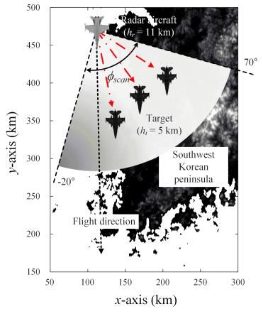
and the water vapor densities for the dry and wet weathers are 0.1 and 18 g/m3 without
           the rainfall. The maximum attenuation values of the dry and wet weather conditions are
           1.4 and 4.9 dB in the range from 0 to 190 km. The dotted and dash-dotted lines denote the
           rainfall attenuations in accordance with the precipitations of 10 mm/hr and 30 mm/hr,
Remote Sens.which   are
             2021, 13,   defined as the normal and heavy rain conditions in this research. The maximum
                       3943                                                                                                             6 of 14
           attenuations in the normal and heavy rainfalls are 5.7 dB at 46.5 km and 15.1 dB at 54 km
           in the range from 0 to 190 km.

                                                             (a)

                                                             (b)

                                                             (c)
         Figure 4. Calculated atmospheric    gas and rainfall
                                 Figure 4. Calculated         attenuation
                                                       atmospheric         results:
                                                                      gas and       (a) rainfall
                                                                               rainfall          attenuation
                                                                                         attenuation  results: accord-
                                                                                                               (a) rainfall attenuation accord-
         ing to frequency; (b) rainfall attenuation according    to precipitation; (c) gas  and  rainfall
                                 ing to frequency; (b) rainfall attenuation according to precipitation;   attenuation
                                                                                                              (c) gas and rainfall attenuation
         according to range.
                                 according to range.

                                       In the atmospheric environment modeling, it is important to consider uncertainties
                                  of the measurement for the atmospheric refractivity [44] and rainfall attenuation, which
                                  can possibly affect the TDP results. For example, if we make an assumption that the
                                  measurement of the refractivity had the uniform uncertainty of 2.5 % along the height, then
                                  the deviations between the original measurement and the uncertainties of the TDP can be
                                  increased up to 4.7% in the long-range over 80 km.
Remote Sens. 2021, 13, 3943                                                                                                 7 of 14

                              2.3. TDP Calculation with Airborne Radar Parameters
                                    In Section 2.1, the refractive index, gas attenuation, rainfall attenuation, and radar
                              parameters were modeled to estimate the total path loss of the wave propagation in an
                              anomalous atmospheric environment; however, more radar parameters and computations
                              are needed to accurately predict the TDP of the airborne radar. We determine the TDP
                              using the threshold evaluations derived from the free-space path loss according to the
                              range. To examine the threshold for the total path loss, the detectability factor is required
                              for a given probability of detection and false alarm as written in Equation (14). In addition,
                              the fluctuation loss is modeled using Equation (15) to calculate the TDP performance for
                              describing the fluctuating target. Finally, these equations are directly related to the radar
                              range equation for the detectable range that is introduced by Blake as follows [45]:
                                                                                             2
                                                            t = 0.9(2Pd − 1), x0 = gd + g f a                                 (15)
                                                                         
                                                                                            r
                                                             1.23t                                      
                                                 gd =  q                 , g f a = 2.36       − log10 Pf a − 1.02           (16)
                                                             1 − ( t )2
                                                                                 s         
                                                                       L f x0          16Np
                                                            D ( Pd ) =        1 + 1 +                                       (17)
                                                                       4Np              x0

                                                                                           1
                                                                L f ( Pd ) =                                                (18)
                                                                                                   gd
                                                                                − ln( Pd ) 1 +     gfa
                                                                          v
                                                                                        c20 Pt στG2
                                                                          u
                                                                          u
                                                                          4
                                                           R f s ( Pd ) = t                                                   (19)
                                                                               (4π )3 kT [ D ( Pd )] f 2 N f Ls

                              where Pd is the detection probability ranging from 0 to 0.99, and Pfa indicates the false
                              alarm rate of the airborne radar. Lf is the fluctuation loss in Swerling Case 1, and Np is
                              the number of pulses integrated by the detector depending on the radar system. D is the
                              detectability factor, and Rfs is the free-space detectable range in meters. c0 is the light speed
                              of 3 × 10⁸ m/s, and σ is the RCS of the target in m2 . k is the Boltzmann constant, and
                              τ is the pulse length of the radar in seconds. Pt and G are transmitting power in watts
                              and the array antenna gain, respectively. Nf and Ls are the noise figure and miscellaneous
                              system loss of the radar. In the radar range Equation (16), it is required to set the system
                              parameters of the airborne radar to specific values: Pt = 1 MW, τ = 2 µs, Pfa = 10−8 , G = 103 ,
                              k = 1.38 × 10⁻²³ , f = 10 GHz, Nf = 100.5 , and Ls = 100.3 . Then, the total path loss of the
                              threshold related to the TDP can be calculated by using the detectable range as follows:
                                                                                                           
                                                                     h            i                        4π
                                                 Ltot ( Pd ) = 20 log R f s ( Pd ) + 20 log( f ) + 20 log                   (20)
                                                                                                           c0

                                   Figure 5 shows the calculated path loss threshold and detectability factor results accord-
                              ing to the detection probability at a fixed RCS value of 8.5 m2 . The path loss threshold varies
                              from 151.4 to 159.2 dB when the Pd increases from 70% to 100%. The maximum detectability
                              factor is 17.9. The total path loss threshold is significantly affected by the detectable range Rfs ,
                              and the detectability factor is dominantly decided by the fluctuation loss for the fluctuating
                              type of the target. To further observe the TDP performance with the ranges and angles, we
                              additionally compute the theoretical scan losses in terms of the scan angle φscan for the beam
                              scanning of the radar array antenna, as written in Equation (18) [46,47].

                                                                          Lscan = cosn (φscan )                               (21)
loss for the fluctuating type of the target. To further observe the TDP performance with
                               loss forwe
            the ranges and angles,        the   fluctuatingcompute
                                              additionally       type of the thetarget.       To further
                                                                                    theoretical     scan losses observe      the TDP
                                                                                                                        in terms     of the  performance with
            scan angle scan for
                               thethe
                                    ranges
                                        beam   and   angles, of
                                                 scanning      wethe additionally
                                                                         radar array     compute
                                                                                            antenna,the   astheoretical
                                                                                                               written in scan         losses in terms of the
                                                                                                                                Equation
Remote Sens.(18)
             2021,[46,47].
                   13, 3943    scan angle scan for the beam scanning of the radar array antenna, as written in Equation                                            8 of 14
                               (18) [46,47].
                                                               Lscan  cos n scan                                                   (21)
                                                                                         Lscan  cos n scan                                                 (21)
            where Lscan is the scan loss of the radar, and n is the power of the cosine function set to be
                                    where Lscan is the scan loss of the radar, and n is the power of the cosine function set to be
                               where
            −2.5 in this research.      Lscan is6athe
                                     Figure            scan loss
                                                    presents      theofscan
                                                                         the loss
                                                                              radar,     and n is to
                                                                                      according       thethepowerscan of    the cosine
                                                                                                                         angle.    Due tofunction set to be
                                    −2.5 in this research. Figure 6a presents the scan loss according to the scan angle. Due
            the beam scanning, the array antenna gain can be gradually attenuated until 6.8 dBthe
                               −2.5  in  this   research.    Figure     6a  presents       the  scan    loss    according        to  at the scan angle. Due to
                                    to the beam scanning, the array antenna gain can be gradually attenuated until 6.8 dB at
            scanning angle of  the70°.
                                    beam Wescanning,
                                               also model   the aarray
                                                                   target antenna
                                                                            aircraftgain  usingcanFEKO
                                                                                                    be gradually
                                                                                                               full EMattenuated
                                                                                                                            software to       until 6.8 dB at the
                                    the scanning angle of 70◦ . We also model a target aircraft using FEKO full EM software to
            obtain the RCSs scanning         angle angles.
                                at the azimuth        of 70°. We Figurealso6bmodel
                                                                                presents a target
                                                                                               the RCSaircraft
                                                                                                            for theusing rearFEKO       full EM software to
                                                                                                                                direction
                                    obtain the RCSs at the azimuth angles. Figure 6b presents the RCS for the rear direction
                               obtainInthe
            of the target aircraft.       theRCSs      at theangle,
                                                scanning        azimuth      angles. Figure
                                                                        the maximum            and 6b     presentsRCS
                                                                                                     averaged            the values
                                                                                                                              RCS for     are the rear direction
                                    of the target aircraft. In the scanning angle, the maximum and averaged RCS values are
            67.2 and 2.8 dBsm  of at
                                  thethe
                                       target
                                           scan aircraft.
                                                  angles ofIn0°   theandscanning
                                                                           70°. With   angle,    the   maximum
                                                                                          the environment                and
                                                                                                                      models    averaged
                                                                                                                                  and     the     RCS values are
                                    67.2 and 2.8 dBsm at the scan angles of 0◦ and 70◦ . With the environment models and the
                               67.2
            radar parameters, weradarand    2.8
                                      can predictdBsm     at the
                                                       the total   scan   angles     of  0°   and  70°.    With     the   environment            models    and the
                                              parameters,      wewave       propagation
                                                                      can predict       the totallosswave
                                                                                                        for the    airborne radar
                                                                                                                propagation         loss in  for the airborne radar
                               radar parameters,
            the air-to-air situation.                     weLtot
                                                              can    predict   the totaltowave        propagation  TDP loss       forEqua-
                                                                                                                                       the airborne radar in
                                    in This    total loss
                                        the air-to-air           is then
                                                            situation.     calculated
                                                                           This   total lossexamine
                                                                                                 Ltot is then the calculated
                                                                                                                           using    to examine the TDP using
                               the air-to-air
            tion (19). For example,     in  the  situation.
                                                 normal        This total loss
                                                             atmospheric             Ltot is then calculated
                                                                               environment,           if the    total topath
                                                                                                                          examine
                                                                                                                               loss   L the
                                                                                                                                         tot isTDP using Equa-
                                    Equation (19). For example, in the normal atmospheric environment,                                           if the total path loss
            147.5 dB at Rt oftion   Ltot is 147.5 dB at Rt of 50 km, then the TDP can be obtained overtotal
                                     (19).
                                50 km,       For
                                           then   example,
                                                  the   TDP     in
                                                               can  the
                                                                      be normal
                                                                          obtained    atmospheric
                                                                                         over    60%      environment,
                                                                                                         regardless        of   if
                                                                                                                               the the
                                                                                                                                     target  60%path     loss Ltot of
                                                                                                                                                     regardless    is the
            RCS. On the other  147.5  dB
                                  hand,     at
                                            the R t of 50
                                                 TDP     forkm,
                                                              very then   the
                                                                      small    TDP
                                                                              targets    can
                                                                                          with be  obtained
                                                                                                  the    RCS      over
                                                                                                                 of  lower 60%
                                    target RCS. On the other hand, the TDP for very small targets with the RCS of lower than   thanregardless
                                                                                                                                       2   m   2      of the target
            (typical military RCS.  2 On
                               airborne)    the   other
                                             dramatically
                                      m2 (typical          hand,
                                                       military     the
                                                                decrease TDP
                                                                    airborne)forforthevery     smalldecrease
                                                                                         long-range
                                                                                 dramatically           targets
                                                                                                           target with
                                                                                                                     over
                                                                                                                    for   thethe
                                                                                                                             100   RCS
                                                                                                                                   km (Loftot lower
                                                                                                                                long-range         targetthan
                                                                                                                                                           over2 100
                                                                                                                                                                 m 2 km
            > 154.2 dB).       (typical
                                    (Ltot military    airborne) dramatically decrease for the long-range target over 100 km (Ltot
                                           > 154.2 dB).
                               > 154.2 dB).
                                                                            Lr =Lscan
                                                      Ltot  LAREPS  Lg Ltot            [dB] + L g + Lr + Lscan [dB] (22)
                                                                                     L AREPS                                                                          (22)
                                                                                   Ltot  LAREPS  Lg  Lr  Lscan [dB]                                        (22)

             Figure 5. Calculated path  loss 5.
                                    Figure   threshold  andpath
                                                Calculated  detectability factorand
                                                                loss threshold   results accordingfactor
                                                                                    detectability   to detection  prob-
                                                                                                         results according to detection proba-
             ability.          Figure   5. Calculated path loss threshold and detectability factor results according to detection prob-
                                    bility.
                               ability.

                                           (a)                                                             (b)
                                                                   (a)                                                             (b)
             Figure 6. Scan loss and target RCS according to scan angle: (a) scan loss according to scan angle; (b)
             RCS of a target aircraft.
                                Figure  6. Scan loss and
                                     Figure  6. Scan  losstarget RCS according
                                                           and target          to scantoangle:
                                                                      RCS according            (a) scan(a)
                                                                                         scan angle:    loss according
                                                                                                           scan         to scan angle;
                                                                                                                loss according  to scan(b)
                                                                                                                                        angle;
                                RCS of a target aircraft.
                                     (b) RCS of a target aircraft.

                                          3. TDP Calculation with Airborne Radar Parameters
                                               Figure 7 shows three air-to-air scenarios considered for the airborne radar TDP simu-
                                          lation in anomalous atmospheric environments. The detailed scenario explanations are as
                                          follows:
                                          (1)     TDPs when azimuth beam scanning within 90◦ in an anomalous atmospheric envi-
                                                  ronment of the refractivity, as shown in Figure 7a.
3. TDP Calculation with Airborne Radar Parameters
                                   Figure 7 shows three air-to-air scenarios considered for the airborne radar TDP sim-
Remote Sens. 2021, 13, 3943   ulation in anomalous atmospheric environments. The detailed scenario explanations  9 of are
                                                                                                                      14
                              as follows:
                               (1) TDPs when azimuth beam scanning within 90° in an anomalous atmospheric envi-
                                   ronment of the refractivity, as shown in Figure 7a.
                              (2) TDPs when azimuth beam scanning within 90◦ in a rainy weather environment, as
                               (2) TDPs when azimuth beam scanning within 90° in a rainy weather environment, as
                                   shown in Figure 7b.
                                   shown
                              (3) TDPs     in Figureto7b.
                                         according     the distance (Rt < 190 km) to the target in a heavy rain environment,
                               (3) as
                                   TDPs   according
                                      shown in Figure to 7c.
                                                         the distance (Rt < 190 km) to the target in a heavy rain environ-
                                   ment, as shown in Figure 7c.

                                               (a)                                (b)                                (c)

                               Figure7.7.Three
                              Figure     Threeair-to-air
                                               air-to-airscenarios
                                                          scenariosfor
                                                                    forthe
                                                                        theTDP
                                                                           TDPsimulation
                                                                                 simulationin
                                                                                            inanomalous
                                                                                               anomalousatmospheric
                                                                                                          atmosphericenvironments:
                                                                                                                      environments:
                               (a)azimuth
                              (a)  azimuthbeam
                                            beamscanning
                                                  scanningininan
                                                               ananomalous
                                                                  anomalousatmospheric
                                                                               atmosphericenvironment;
                                                                                            environment;(b)
                                                                                                          (b)azimuth
                                                                                                              azimuthbeam
                                                                                                                      beamscanning
                                                                                                                           scanning
                               in a rainy environment;   (c) encountering  a target in a heavy rain environment.
                              in a rainy environment; (c) encountering a target in a heavy rain environment.

                                   In
                                    Inall
                                       allscenarios,
                                           scenarios,the       heighthhr rof
                                                         theheight         ofthe
                                                                              theairborne
                                                                                  airborneradar
                                                                                              radarisisconsistent
                                                                                                        consistentatat11 11km,
                                                                                                                            km,and
                                                                                                                                 andthe
                                                                                                                                      the
                              target  height h   is set   to  be 5 km.     Additionally,    these  scenarios   are  in  the
                               target height ht is set to be 5 km. Additionally, these scenarios are in the long-range radar
                                               t                                                                            long-range
                              radar  propagation
                               propagation          situations,
                                             situations,    which which
                                                                    assumesassumes    thatslant
                                                                                that the   the slant
                                                                                                rangerange   is almost
                                                                                                        is almost  samesamewithwith  the
                                                                                                                                the hori-
                               zontal range (Rt  R
                              horizontal  range  (R   ≈  R h detailed explanations for the scenarios are listed in Table 2. 2.
                                                    t h). The). The detailed   explanations    for the scenarios  are  listed in Table

                               Table2.2.TDP
                              Table      TDPsimulation
                                             simulationscenarios.
                                                        scenarios.

                                                                  Scenario
                                                               Scenario   I I             Scenario
                                                                                     Scenario      II II              Scenario III
                                                                                                                    Scenario    III
                                    Scan  range(R(R
                                    Scan range     t )t)    0 km–190
                                                                   0–190 km
                                                                         km         0 km–190
                                                                                           0–190km  km             0 km–190
                                                                                                                       0–190 km km
                               Elevation steeringangle
                                Elevation steering     angle         −4.3◦
                                                                  −4.3°                      −4.3◦
                                                                                         −4.3°                         −1.8–31◦
                                                                                                                       −1.8–31°
                                   Scan angle (φscan )             −20–70  ◦               −20–70     ◦                    0◦
                                   Scan angle (scan)           −20–70°                −20–70°                            0°
                                                             Normal (∇M = 85)
                                Atmospheric condition       Normal
                                                               Sub (∇(M     =
                                                                       M = 300)       Normal (∇M = 85)
                                                                                                                  Normal (∇M = 85)
                                         (∇M)                      85)(∇M = 10)
                                                               Super                   Super (∇M = 10)
                               Atmospheric condition Sub         (M(∇
                                                            Ducting    =M  = −80)Normal (M = 85)
                                                                         300)
                                                                                                         3       Normal   (M    = 385)
                                          (M)             Super (M = 10)3       SuperDry(M(0.1=g/m
                                                                                                    10) )           Dry (0.1  g/m    )
                                  Weather condition (e)         Dry (0.1 g/m )              Rainfall                 Heavy rainfall
                                                            Ducting (M =                 (12 mm/h)                   (22 mm/h)
                                                                  −80)
                                                                                   Dry (0.1 g/m3)                  Dry (0.1 g/m3)
                                   Figure 8a illustrates the simulation results   of the TDP    along    the   range and the azimuth
                                 Weather condition (e) Dry (0.1 g/m3)                  Rainfall                    Heavy rainfall
                              angle for the first scenario, where the deep red and blue colors indicate the TDP of 100%
                              and 0%. The TDP over 90% is obtained at the scan       (12angle
                                                                                         mm/hr)  of 0◦ due to the(22     mm/hr)
                                                                                                                       high  RCS level
                              of the target aircraft, and  P t = 1 MW, τ = 2 μs, Pfa = 10−8, G = 103, k = 1.38×10⁻²³, f = 10 GHz,
                                                           the  target  is detected  over  the    probability     of 80%   in  the scan
                                   Radar parameter
                              angle between −20◦ and 60◦ and the range from          Nf 50.5
                                                                                        = 100.5
                                                                                              to, L153.8
                                                                                                    s = 10km.
                                                                                                           0.3.
                                                                                                                  On the other hand,
                              the range from 0 to 50.2 km within the whole scan angle has the low TDP because this
                              is the area below the airborne radar beam that cannot be reached. In addition, the scan
                              loss of the airborne radar increases the path loss, which reduces the TDP in the wide
                              angle from 60◦ to 90◦ . Figure 8b depicts the contour plot of the TDP over the 90% region
                              according to the different atmospheric conditions of the refractivity. The solid, dashed,
                              dotted, and dash-dotted lines denote the normal refraction, super-refraction, sub-refraction,
                              and elevated ducting cases. We defined a detectable area by calculating the area inside
                              the contour region to intuitively examine the TDP. The resulting detectable area of the
range from 0 to 50.2 km within the whole scan angle has the low TDP because this is the
                       area below the airborne radar beam that cannot be reached. In addition, the scan loss of
                       the airborne radar increases the path loss, which reduces the TDP in the wide angle from
                       60° to 90°. Figure 8b depicts the contour plot of the TDP over the 90% region according to
                       the13,
        Remote Sens. 2021, different
                              3943    atmospheric conditions of the refractivity. The solid, dashed, dotted, and              10 of 14
                       dash-dotted lines denote the normal refraction, super-refraction, sub-refraction, and ele-
                       vated ducting cases. We defined a detectable area by calculating the area inside the con-
                       tour region to intuitively examine the TDP. The resulting detectable area of the super-
                                          super-refraction is larger than those of the others, which are similar to each other. It is
                       refraction is larger than those of the others, which are similar to each other. It is because
                                          because the super-refraction makes the wave propagation bend toward Earth’s surface,
                       the super-refraction makes the wave propagation bend toward Earth’s surface, which re-
                                          which results in low path loss levels over a large area. The summary of the detectable area
                       sults in low path loss levels over a large area. The summary of the detectable area results
                                          results for TDPs over 80% and 90% is shown in Figure 8c.
                       for TDPs over 80% and 90% is shown in Figure 8c.

                                                                        (a)

2021, 13, x FOR PEER REVIEW                                                                                            11 of 14

                                                                        (b)

                                                                       (c)
                    Figure 8. Simulation Figure
                                          results 8.
                                                  of Simulation
                                                     the TDP along   the of
                                                                 results range  and the
                                                                            the TDP     azimuth
                                                                                     along       angle
                                                                                           the range   forthe
                                                                                                     and   theazimuth
                                                                                                               first scenario:
                                                                                                                        angle for the first scenario:
                    (a) TDP in a super-refraction; (b) contour plots of TDP in an anomalous atmospheric environment;
                                          (a) TDP in a super-refraction; (b) contour plots of TDP in an anomalous atmospheric environment;
                    (c) detectable area results for TDPs over 80% and 90%.
                                          (c) detectable area results for TDPs over 80% and 90%.

                         Figure 9 illustrates the contour plot of the TDP over 80% according to the different
                    weather conditions in the sub- and normal refractions for the second scenario. The solid
                    and dashed lines indicate the TDP results according to the dry and rainy weather in the
                    normal atmospheric condition, while the dotted and dash-dotted lines denote the results
                    in the amorous atmospheric condition (super-refraction). In the dry weather, the TDP for
(c)
         RemoteFigure  8. Simulation
                Sens. 2021, 13, 3943 results of the TDP along the range and the azimuth angle for the first scenario:                  11 of 14
              (a) TDP in a super-refraction; (b) contour plots of TDP in an anomalous atmospheric environment;
              (c) detectable area results for TDPs over 80% and 90%.

                                              Figure plot
                   Figure 9 illustrates the contour    9 illustrates
                                                             of the TDPthe contour
                                                                            over 80%plot   of the TDP
                                                                                       according         over
                                                                                                    to the     80% according to the different
                                                                                                            different
              weather conditions in the sub- and normal refractions for the second scenario. Thethe
                                         weather   conditions    in the  sub-  and normal     refractions  for      second scenario. The solid
                                                                                                                solid
              and dashed lines indicate the TDP results according to the dry and rainy weather in theand rainy weather in the
                                         and  dashed    lines indicate    the TDP  results   according   to the  dry
                                         normalwhile
              normal atmospheric condition,       atmospheric     condition,
                                                         the dotted            while thelines
                                                                      and dash-dotted      dotted   and dash-dotted
                                                                                                  denote  the results lines denote the results
                                         in the amorous     atmospheric     condition   (super-refraction).
              in the amorous atmospheric condition (super-refraction). In the dry weather, the TDP            In the
                                                                                                                   fordry weather, the TDP for
                                         the normal
              the normal and super-refractions         and super-refractions
                                                    is similar  to the results ofisthe
                                                                                    similar
                                                                                         first to the results
                                                                                               scenario,  whereof the
                                                                                                                  the first scenario, where the
                                         detectable   areas are  4738  and   6298 km 2 , respectively. In contrast, in rainy weather, the TDP
              detectable areas are 4738 and 6298 km , respectively. In contrast, in rainy weather, the TDP
                                                        2
                                         of the airborne
              of the airborne radar is extremely            radar is because
                                                      deteriorated     extremelyof deteriorated     because of the
                                                                                   the rainfall attenuation.      Therainfall attenuation. The
                                         resulting  detectable   areas   for
              resulting detectable areas for the normal and super-refraction the normal    and  super-refraction
                                                                                     atmospheric environments       atmospheric environments
                                         are 1670  and    1734  km  2 . Note that the rainfall loss considerably affects the TDP of the
              are 1670 and 1734 km2. Note that the rainfall loss considerably affects the TDP of the air-
                                         airborne radar. In the third scenario, we additionally simulate and calculate the TDP of the
              borne radar. In the third scenario, we additionally simulate and calculate the TDP of the
                                         airborne radar using another wave propagation simulation software (PETOOL) based on
              airborne radar using another wave propagation simulation software (PETOOL) based on
                                         one-way and two-way split-step parabolic equation [48] and the ITU-R P.528-4 model [49]
              one-way and two-way split-step parabolic equation [48] and the ITU-R P.528-4 model [49]
                                         to confirm the results of the proposed process. Figure 10 shows the comparison of the TDP
              to confirm the results of the proposed process. Figure 10 shows the comparison of the TDP
                                         results along the target range of Rt using the different propagation models for the third
              results along the target range of Rt using the different propagation            models for the third
                                         scenario when the target and the airborne radar are gradually getting closer to each other.
              scenario when the target and the airborne radar are gradually getting closer to each other.
                                         The airborne radar TDP becomes significantly low (almost zero TDP) when the heavy
              The airborne radar TDP becomes significantly low (almost zero TDP) when the heavy
                                         rainfall occurs. In the target range of Rt below 100 km, the AREPS simulation result well
              rainfall occurs. In the target range of Rt below 100 km, the AREPS simulation result well
                                         agrees with those of the PETOOL and ITU-R model. These results demonstrate that the
              agrees with those of the PETOOL and ITU-R model. These results demonstrate that the
                                         proposed process is feasible for observing the TDP of the airborne radar considering the
              proposed process is feasible for observing the TDP of the airborne radar considering the
                                         anomalous atmospheric environments.
              anomalous atmospheric environments.

3, x FOR PEER REVIEW                      Figure
               Figure 9. Contour plot of TDP     9. Contour
                                              according     plot of TDP
                                                        to different     according
                                                                     weather       to different
                                                                             conditions         weather
                                                                                        in the sub-      12 of 14
                                                                                                    and conditions
                                                                                                        normal     in the sub- and normal
                                           refractions for the second scenario.
              refractions for the second scenario.

               Figure 10. Comparison of TDP  along
                                        Figure     the range using
                                               10. Comparison      different
                                                               of TDP  alongpropagation models
                                                                             the range using     for thepropagation
                                                                                             different    third     models for the third
               scenario.                scenario.

               4. Conclusions              4. Conclusions
                                            In the
                    In this paper, we proposed  thisTDP
                                                     paper,  we proposed
                                                        calculation processthe TDP
                                                                            using  thecalculation process using the airborne long-
                                                                                       airborne long-range
                                        range radar  path  loss based on the  air-to-air scenarios in anomalous atmospheric and
               radar path loss based on the air-to-air scenarios in anomalous atmospheric and weather
               environments. The refractive index along an altitude was modeled using a quad-linear
               model. Then, the path loss including the refractivity model and other radar input param-
               eters was simulated using the AREPS software along the range and the altitude. ITU-R
               models were used to consider the weather environment for the gas and rainfall attenua-
Remote Sens. 2021, 13, 3943                                                                                                          12 of 14

                                   weather environments. The refractive index along an altitude was modeled using a quad-
                                   linear model. Then, the path loss including the refractivity model and other radar input
                                   parameters was simulated using the AREPS software along the range and the altitude.
                                   ITU-R models were used to consider the weather environment for the gas and rainfall
                                   attenuations according to the range. In addition, the radar beam scan loss and RCS of
                                   the target were considered to estimate the TDP of the airborne long-range radar. Various
                                   air-to-air scenarios were assumed for the airborne radar TDP simulation in the anomalous
                                   atmospheric and weather environments. In the first scenario, the target was detected over
                                   the probability of 80% in the scan angle between −20◦ and 60◦ and the range from 50.5 to
                                   153.8 km. In the second scenario, the TDP of the airborne radar was extremely deteriorated
                                   in the rainfall weather because of the rainfall attenuation. The resulting detectable areas
                                   for the normal and super-refraction atmospheric environments were 1670 and 1734 km2 . In
                                   the third scenario, the airborne radar TDP became significantly low due to the rainfall.

                                   Author Contributions: Conceptualization, T.-H.L. and H.C.; methodology, T.-H.L. and H.C.; soft-
                                   ware, T.-H.L.; validation, T.-H.L. and H.C.; formal analysis, T.-H.L. and H.C.; investigation, T.-H.L.
                                   and H.C.; resources, T.-H.L. and H.C.; data curation, T.-H.L.; writing—original draft preparation,
                                   T.-H.L.; writing—review and editing, H.C.; visualization, T.-H.L. and H.C.; supervision, H.C.; project
                                   administration, H.C.; funding acquisition, H.C. All authors have read and agreed to the published
                                   version of the manuscript.
                                   Funding: This research received no external funding.
                                   Institutional Review Board Statement: Not applicable.
                                   Informed Consent Statement: Informed consent was obtained from all subjects involved in the study.
                                   Data Availability Statement: Not applicable.
                                   Acknowledgments: This work was supported by a grant-in-aid of HANWHA SYSTEMS. This
                                   work was supported by the National Research Foundation of Korea (NRF) grant funded by the
                                   Korea government (MSIT) (NRF-2017R1A5A1015596). This research was supported by Basic Science
                                   Research Program through the National Research Foundation of Korea (NRF) funded by the Ministry
                                   of Education (No. 2015R1A6A1A03031833).
                                   Conflicts of Interest: The authors declare no conflict of interest.

References
1.    Rim, J.-W.; Koh, I.-S. SAR image generation of ocean surface using time-divided velocity bunching model. J. Electromagn. Eng. Sci.
      2019, 19, 82–88. [CrossRef]
2.    Farina, A.; Saverione, A.; Timmoneri, L. MVDR vectorial lattice applied to space–time processing for AEW radar with large
      instantaneous bandwidth. IEE Proc.-Radar Sonar Navig. 1996, 143, 41–46. [CrossRef]
3.    Kim, E.H.; Park, J. Dwell time optimization of alert-confirm detection for active phased array radars. J. Electromagn. Eng. Sci.
      2019, 19, 107–114. [CrossRef]
4.    Nam, J.-H.; Rim, J.-W.; Lee, H.; Koh, I.-S.; Song, J.-H. Modeling of monopulse radar signals reflected from ground clutter in a time
      domain considering doppler effects. J. Electromagn. Eng. Sci. 2020, 20, 190–198. [CrossRef]
5.    Benzon, H.; Høeg, P. Wave propagation simulation of radio occultations based on ECMWF refractivity profiles. Radio Sci. 2015,
      50, 778–788. [CrossRef]
6.    Barclay, M.; Pietzschmann, U.; Gonzalez, G.; Tellini, P. AESA upgrade option for Eurofighter captor radar. IEEE Aerosp. Electron.
      Syst. Mag. 2010, 25, 11447006. [CrossRef]
7.    Mesnard, F.; Sauvageot, H. Climatology of anomalous propagation radar echoes in a coastal area. J. Appl. Meteorol. Climatol. 2010,
      49, 2285–2300. [CrossRef]
8.    Lenouo, A. Climatology of anomalous propagation radar over Douala, Cameroon. Meteorol. Appl. 2014, 21, 249–255. [CrossRef]
9.    Colussi, L.C.; Schiphorst, R.; Teinsma, H.W.M.; Witvliet, B.A.; Fleurke, S.R.; Bentum, M.J.; van Maanen, E.; Griffioen, J. Multiyear
      trans-horizon radio propagation measurements at 3.5 ghz. IEEE Trans. Antennas Propag. 2018, 66, 884–896. [CrossRef]
10.   López, R.N.; del Río, V.S. High temporal resolution refractivity retrieval from radar phase measurements. Remote Sens. 2018, 10,
      896. [CrossRef]
11.   Wang, L.; Wei, M.; Yang, T.; Liu, P. Effects of atmospheric refraction on an airborne weather radar detection and correction
      method. Adv. Meteorol. 2015, 2015, 407867. [CrossRef]
12.   Gerstoft, P.; Rogers, L.T.; Krolik, J.L.; Hodgkiss, W.S. Inversion for refractivity parameters from radar sea clutter. Radio Sci. 2003,
      38, 8053. [CrossRef]
Remote Sens. 2021, 13, 3943                                                                                                         13 of 14

13.   Lowry, A.R.; Rocken, C.; Sokolovskiy, S.V.; Anderson, K.D. Vertical profiling of atmospheric refractivity from ground-based GPS.
      Radio Sci. 2002, 37, 1–19. [CrossRef]
14.   Liu, X.; Wu, Z.; Wang, H. Inversion method of regional range-dependent surface ducts with a base layer by doppler weather
      radar echoes based on WRF model. Atmosphere 2020, 11, 754. [CrossRef]
15.   Wagner, M.; Gerstoft, P.; Rogers, T. Estimating refractivity from propagation loss in turbulent media. Radio Sci. 2016, 51, 1876–1894.
      [CrossRef]
16.   Gunashekar, S.D.; Warrington, E.M.; Siddle, D.R.; Valtr, P. Signal strength variations at 2 GHz for three sea paths in the British
      Channel Islands: Detailed discussion and propagation modeling. Radio Sci. 2007, 42, 1–13. [CrossRef]
17.   Wang, Q.; Alappattu, D.P.; Billingsley, S.; Blomquist, B.; Burkholder, R.J.; Christman, A.J.; Creegan, E.D.; Paolo, T.; de Eleuterio,
      D.P.; Fernando, H.J.S.; et al. CASPER: Coupled air–sea processes and electromagnetic ducting research. Bull. Am. Meteorol. Soc.
      2018, 99, 1449–1471. [CrossRef]
18.   Habib, A.; Moh, S. Wireless channel models for over-the-sea communication: A comparative study. Appl. Sci. 2019, 9, 443.
      [CrossRef]
19.   Shi, Y.; Kun-De, Y.; Yang, Y.-X.; Ma, Y.-L. Influence of obstacle on electromagnetic wave propagation in evaporation duct with
      experiment verification. Chin. Phys. B 2015, 24, 054101. [CrossRef]
20.   Wang, S.; Lim, T.H.; Chong, Y.J.; Ko, J.; Park, Y.B.; Choo, H. Estimation of abnormal wave propagation by a novel duct map based
      on the average normalized path loss. Microw. Opt. Technol. Lett. 2020, 62, 1662–1670. [CrossRef]
21.   Barrios, A.E. Considerations in the development of the advanced propagation model (APM) for U.S. Navy applications. In
      Proceedings of the 2003 International Conference on Radar, Adelaide, SA, Australia, 3–5 September 2003; pp. 77–82.
22.   Sirkova, I. Brief review on PE method application to propagation channel modeling in sea environment. Open Eng. 2012, 2, 19–38.
      [CrossRef]
23.   Levy, M. Parabolic Equation Methods for Electromagnetic Wave Propagation; The Institution of Engineering and Technology: London,
      UK, 2000.
24.   Hardin, R.H.; Tappert, F.D. Application of the split-step Fourier method to the numerical solution of nonlinear and variable
      coefficient wave equations. SIAM Rev. 1973, 15, 423.
25.   Ozgun, O. New Software Tool (GO+UTD) for visualization of wave propagation [testing ourselves]. IEEE Antennas Propag. Mag.
      2016, 58, 91–103. [CrossRef]
26.   Patterson, W.L. User Manual for Advanced Refractive Effects Prediction System (AREPS); Space Naval Warfare System Center: San
      Diego, CA, USA, 2004.
27.   Schwartz, B.; Benjamin, S.G. A comparison of temperature and wind measurements from ACARS-equipped aircraft and
      Rawinsondes. Weather Forecast. 1995, 10, 528–544. [CrossRef]
28.   Lee, T.R.; Pal, S. On the potential of 25 years (1991–2015) of rawinsonde measurements for elucidating climatological and
      spatiotemporal patterns of afternoon boundary layer depths over the contiguous US. Adv. Meteorol. 2017, 2017, 6841239.
      [CrossRef]
29.   Hock, T.F.; Franklin, J.L. The NCAR GPS dropwindsonde. Bull. Amer. Meteorol. Soc. 1999, 80, 407–420. [CrossRef]
30.   ITU. The Radio Refractive Index: Its Formula and Refractivity Data. Available online: https://www.itu.int/rec/R-REC-P.453/en
      (accessed on 24 August 2021).
31.   Korea Meteorological Administration. Available online: https://www.kma.go.kr/eng/index.jsp (accessed on 24 August 2021).
32.   Lim, T.H.; Go, M.; Seo, C.; Choo, H. Analysis of the target detection performance of air-to-air airborne radar using long-range
      propagation simulation in abnormal atmospheric conditions. Appl. Sci. 2020, 10, 6440. [CrossRef]
33.   National Geographic Information Institute. Available online: https://www.ngii.go.kr/eng/main.do? (accessed on 24 August
      2021).
34.   ITU. Attenuation by Atmospheric Gases and Related Effects. Available online: https://www.itu.int/rec/R-REC-P.676-12-201908-
      I/en (accessed on 24 August 2021).
35.   ITU. Propagation Data and Prediction Methods Required for the Design of Terrestrial Line-of-Sight Systems. 2017. Available
      online: https://www.itu.int/rec/R-REC-P.530-17-201712-I (accessed on 24 August 2021).
36.   ITU. Characteristics of Precipitation for Propagation Modelling, International Telecommunication Union 2017. Available online:
      https://www.itu.int/rec/R-REC-P.837-7-201706-I/en (accessed on 24 August 2021).
37.   ITU. Specific Attenuation Model for Rain for Use in Prediction Methods 2005. Available online: https://www.itu.int/rec/R-REC-
      P.838-3-200503-I/en (accessed on 24 August 2021).
38.   Shayea, I.; Rahman, T.A.; Azmi, M.H.; Islam, R. Real measurement study for rain rate and rain attenuation conducted over 26 Ghz
      microwave 5G link system in Malaysia. IEEE Access 2018, 6, 19044–19064. [CrossRef]
39.   Nalinggam, R.; Ismail, W.; Singh, M.J.; Islam, M.T.; Menon, P.S. Development of rain attenuation model for Southeast Asia
      equatorial climate. IET Commun. 2013, 7, 1008–1014. [CrossRef]
40.   Shrestha, S.; Choi, D.-Y. Rain attenuation study over an 18 GHz terrestrial microwave link in South Korea. Int. J. Antennas Propag.
      2019, 2019, 1712791. [CrossRef]
41.   Shebani, N.M.; Kaeib, A.F.; Zerek, A.R. Estimation of rain attenuation based on ITU-R model for terrestrial link in Libya. In
      Proceedings of the 5th International Conference of Control Signal Processing, Kairouan, Tunisia, 28–30 October 2017.
Remote Sens. 2021, 13, 3943                                                                                                       14 of 14

42.   Kestwal, M.C.; Joshi, S.; Garia, L.S. Prediction of rain attenuation and impact of rain in wave propagation at microwave frequency
      for tropical region (Uttarakhand, India). Int. J. Microw. Sci. Technol. 2014, 2014, 958498. [CrossRef]
43.   Islam, R.; Rahman, T.A.; Karfaa, Y. Worst-month rain attenuation statistics for radio wave propagation study in Malaysia. In
      Proceedings of the 9th Asia-Pacific Conference on Communications, Penang, Malaysia, 21–24 September 2003; Volume 3, pp.
      1066–1069.
44.   Jicha, O.; Pechac, P.; Kvicera, V.; Grabner, M. On the uncertainty of refractivity height profile measurements. IEEE Antennas Wirel.
      Propag. Lett. 2011, 10, 983–986. [CrossRef]
45.   Blake, L.V. Radar Range-Performance Analysis; Munro Pub. Co.: Silver Spring, MD, USA, 1991.
46.   Mailloux, R.J. Phased Array Antenna Handbook, 3rd ed.; Artech House: Norwood, MA, USA, 2018.
47.   Nathanson, F.E.; O’Reilly, P.J.; Cohen, M.N. Radar Design Principles: Signal Processing and the Environment; Scitech Publ.: Raleigh,
      NC, USA, 2004.
48.   Ozgun, O.; Apaydin, G.; Kuzuoglu, M.; Sevgi, L. PETOOL: MATLAB-based one-way and two-way split-step parabolic equation
      tool for radiowave propagation over variable terrain. Comput. Phys. Commun. 2011, 182, 2638–2654. [CrossRef]
49.   ITU. A Propagation Prediction Method for Aeronautical Mobile and Radionavigation Services Using the VHF, UHF and SHF
      Bands 2019. Available online: https://www.itu.int/rec/R-REC-P.528-4-201908-I/en (accessed on 24 August 2021).
You can also read