PRICE SETTING IN ONLINE MARKETS: DOES IT CLICK? - Econometrics ...
←
→
Page content transcription
If your browser does not render page correctly, please read the page content below
PRICE SETTING IN ONLINE MARKETS:
DOES IT CLICK?

Yuriy Gorodnichenko                                  Viacheslav Sheremirov
University of California, Berkeley and               Federal Reserve Bank of Boston
NBER
Oleksandr Talavera
Swansea University

Abstract
Using a unique dataset of daily U.S. and U.K. price listings and the associated number of clicks for
precisely defined goods from a major shopping platform, we shed new light on how prices are set
in online markets, which have a number of special properties such as low search costs, low costs
of monitoring competitors’ prices, and low costs of nominal price adjustment. We document that
although online prices change more frequently than offline prices, they nevertheless exhibit relatively
long spells of fixed prices. By many metrics, such as large size and low synchronization of price
changes, considerable cross-sectional dispersion, and low sensitivity to predictable or unanticipated
changes in demand conditions, online prices are as imperfect as offline prices. Our findings suggest
a need for more research on the sources of price rigidities and dispersion, as well as on the relative
role of menu and search costs in online-pricing frictions. (JEL: E31, L11, L86)

1. Introduction

Internet firms such as Google, Amazon, and eBay are revolutionizing the retail
sector, as there has been an explosion in the volume and coverage of goods and

The editor in charge of this paper was Claudio Michelacci.
Acknowledgments: We are grateful to Hal Varian for his support and comments, as well as to the
editor, anonymous referees, Eric Bartelsman (discussant), Alberto Cavallo (discussant), Jeff Fuhrer,
Sergei Koulayev, Ricardo Nunes, Ali Ozdagli, and seminar participants at UC Berkeley GEMS; NBER
Summer Institute’s Price Dynamics group; Royal Economic Society meeting; 14th EBES conference;
1st International Conference in Applied Theory, Macro, and Empirical Finance; Federal Reserve Bank
of Boston; UC Irvine; UC Santa Cruz; Federal Reserve Board of Governors; NBER International
Comparisons of Income, Prices, and Production at MIT Sloan; and 19th annual De Nederlandsche
Bank research conference for comments and discussion. Gorodnichenko thanks the NSF and the Sloan
Foundation for financial support. Sandra Spirovska and Nikhil Rao provided excellent research assistance.
We thank Oleksiy Kryvtsov and Nicolas Vincent for sharing their data. We are also grateful to Suzanne
Lorant and Stephanie Bonds for superb editorial assistance. The views expressed herein are those of the
authors and are not necessarily those of the Federal Reserve Bank of Boston or the Federal Reserve System.
E-mail: ygorodni@econ.berkeley.edu (Gorodnichenko); viacheslav.sheremirov@bos.frb.org
        (Sheremirov); oleksandr.talavera@gmail.com (Talavera)

Journal of the European Economic Association
Preprint prepared on September 19, 2017 using jeea.cls v1.0.
Gorodnichenko, Sheremirov, and Talavera             Price Setting in Online Markets                          2

services sold online. In 2013, Amazon alone generated $74.5 billion in revenue—
approximately the revenue of Target Corporation, the second largest discount retailer
in the United States—and carried 230 million items for sale in the United States—
nearly 30 times the number sold by Walmart, the largest retailer in the world. While
virtually nonexistent 15 years ago, according to the New York Times, “[i]n the last three
months of 2016, Americans spent $102.7 billion in online sales, which was 8.3% of
the overall total of $1.24 trillion in retail sales.”1 The rise of e-commerce has been
truly a global phenomenon, and global e-commerce sales are expected to reach $4
trillion by 2020 (Statista 2016). While visionaries of the internet age are utterly bold
in their predictions, one can already exploit special properties of online retail, such
as seemingly low search costs, low costs of monitoring competitors’ prices, and low
costs of nominal price adjustment (Ellison and Ellison 2005), to shed new light on
some perennial questions in economics and the workings of future markets.
     We use a unique dataset of daily price listings for precisely defined goods (at the
level of unique product codes) from a major online shopping platform to examine price
setting practices in online markets in the United States and the United Kingdom, two
countries with a developed internet retail industry. This dataset covers an exceptionally
broad spectrum of consumer goods and sellers over a period of nearly two years.
Similar to the dataset in Gorodnichenko and Talavera (2017), these data pertain to an
online-shopping/price-comparison website, a growing gateway for internet commerce.
However, in contrast to Gorodnichenko and Talavera (2017) and others who scraped
websites to collect their data, we have data directly provided by the platform, which
allows us to have the unprecedented quality of information characterizing online
markets. Most importantly, this dataset represents a stratified random sample of all
goods and sellers on the platform. It also expands product coverage tremendously,
bringing it significantly closer to that in the CPI and giving us more room to compare
online and offline prices.2 Finally, we have the number of clicks for each price listing
so that, in contrast to previous works, we can identify and study prices relevant to
consumers.
     This paper’s objective is to document an extensive set of the empirical properties of
online prices (such as the frequency and size of price changes, price synchronization
across sellers and across goods, cross-store price dispersion, and price responses to

1. “From ‘Zombie Malls’ to Bonobos: What America’s Retail Transformation Looks Like,”
by J. Taggart and K. Granville. The New York Times from 4/15/2017. Available online at
https://www.nytimes.com/2017/04/15/business/from-zombie-malls-to-bonobos-americas-retail-
transformation.html.
2. Gorodnichenko and Talavera (2017) have longer time series (five years of online price data) and
detailed descriptions of goods, but the coverage of goods is limited to electronics, cameras, computers, and
software. Note that because Gorodnichenko and Talavera (2017) study cross-country price differentials,
they focus on goods sold in multiple countries, which is a relatively small subset of goods sold within a
country. Also the platform used in this paper is larger than the platform in Gorodnichenko and Talavera
(2017) or any other study. Gorodnichenko and Talavera (2017)—and similar studies—report only a subset
of statistics covered in the present paper. Despite differences in the sample of goods, time periods, etc., the
results in this paper are broadly similar to the results reported in Gorodnichenko and Talavera (2017).

Journal of the European Economic Association
Preprint prepared on September 19, 2017 using jeea.cls v1.0.
Gorodnichenko, Sheremirov, and Talavera         Price Setting in Online Markets         3

predictable changes in demand) and to compare our findings to results reported for
price data from conventional, brick-and-mortar stores. Similarities or differences in
the properties of prices across online and offline stores inform us about the nature and
sources of sluggish price adjustment, price discrimination, price dispersion, and many
other important dimensions of market operation. Empirical regularities documented
in this paper are compared to the predictions of existing theories of price setting and,
thus, provide critical inputs for future theoretical work on the matter.
     Our main result is that, despite the power of the internet, online price setting
is characterized by considerable frictions. By many metrics, such as the size and
synchronization of price changes, price dispersion, or sensitivity to changes in
economic conditions, the magnitude of these frictions should be similar to that in
offline price setting. However, we also find significant quantitative differences: the
frequency of price changes is higher online than offline. These results continue to
hold when we compare the properties of online and offline prices for narrowly defined
product categories, which ensures that the composition of goods is similar across
markets. Jointly, these facts call for more research on the relative importance of menu,
information, and search costs—and, more generally, on the price-setting mechanism
in online markets.
     Specifically, we find that, despite small physical costs of price adjustment and
reduced costs of collecting and processing information, the duration of price spells
in online markets is about 7 to 20 weeks, depending on the treatment of sales. While
this duration is considerably shorter than the duration typically reported for prices in
brick-and-mortar stores, online prices clearly do not adjust every instant. The median
absolute size of a price change in online markets, another measure of price stickiness,
is 11% in the United States and 5% in the United Kingdom, comparable to the size of
price changes in offline stores. Sales in online markets are about as frequent as sales in
conventional stores (the share of goods on sale is approximately 1.5%–2% per week)
but the average size of sales (10%–12% or less in the United States and 6% or less in
the United Kingdom) is considerably smaller. We use rich, cross-sectional variation of
market and good characteristics to analyze how they are related to various pricing
moments. We find, for example, that the degree of price rigidity is smaller when
markets are more competitive; that is, with a larger number of sellers, the frequency
of price changes increases and the median size decreases.
     Although the costs of monitoring competitors’ prices and the costs of search
for better prices are extraordinarily low in online markets, we observe little
synchronization of price changes across sellers, another key statistic for non-neutrality
of nominal shocks, a finding inconsistent with simultaneously low costs of monitoring
competitors’ prices and low costs of search for better prices. In particular, the
synchronization rate is approximately equal to the frequency of price adjustment,
suggesting that, by and large, online firms adjust their prices independently of their
competitors. Even over relatively long horizons, synchronization is low. We also fail
to find strong synchronization of price changes across goods within a seller; that
is, a typical seller does not adjust prices of its goods simultaneously. Finally, the

Journal of the European Economic Association
Preprint prepared on September 19, 2017 using jeea.cls v1.0.
Gorodnichenko, Sheremirov, and Talavera         Price Setting in Online Markets                  4

synchronization rates of sales across goods for a given seller and across sellers for
a given good are similar to the frequency of sales.
     In line with Warner and Barsky (1995), we find some evidence that prices in online
stores respond to seasonal changes in demand during Thanksgiving and Christmas,
which is similar to the behavior of prices in regular stores. We also show that there
is large variation in demand, proxied by the number of clicks, over days of the week
or month. For example, there are 33% more clicks on Mondays than on Saturdays.
Yet, online prices appear to have little, if any, reaction to these predictable changes
in demand, a finding that is inconsistent with the predictions of Warner and Barsky
(1995). These findings are striking because online stores are uniquely positioned to
use dynamic pricing (i.e., instantaneously incorporate information about changes in
demand and supply conditions).
     We document ubiquitous price dispersion in online markets. For example, the
standard deviation of log prices for narrowly defined goods is 23.6 log points in the
United States and 21.3 log points in the United Kingdom. Even after removing seller
fixed effects, which proxy for differences in terms of sales across stores, the dispersion
remains large. We also show that this high price dispersion cannot be rationalized
by product life cycle. Specifically, a chunk of price dispersion appears at the time a
product enters the market and price dispersion grows (rather than falls) as the product
becomes older. Price dispersion appears to be best characterized as spatial rather than
temporal. In other words, if a store charges a high price for a given good, it does so
consistently over time rather than alternating the price between low and high levels.
In addition, price dispersion can be related to the degree of price stickiness, intensity
of sales, and returns to search.
     To underscore the importance of clicks, we also calculate and present all moments
weighted by clicks. Such weighting tends to yield results consistent with a greater
flexibility of online markets relative to conventional markets: price rigidities decline,
cross-sectional price dispersion falls, synchronization of price changes increases. For
example, using weights reduces the median duration of price spells from 7–12 to 5–
7 weeks. Yet, even when we use click-based weights, online markets are far from
completely flexible.
     Comparing prices in the United States and the United Kingdom offers additional
insights.3 High penetration of online trade in the two countries is largely due to
availability of credit cards, a history of mail order and catalogue shopping, and an early
arrival of e-retailers, such as Amazon and eBay. Yet, there are important differences
between the two markets. For example, population density is eight times higher in
the United Kingdom than in the United States; thus, it is easier to organize fast
and frequent deliveries in the United Kingdom. We find that, despite the differences
between the markets, price setting behavior is largely the same in the two countries.

3. In 2011 (median year in our sample), the value per head of business-to-consumer (B2C) e-commerce
in the United Kingdom was £1,083, making it the leading nation in terms of e-commerce. The growth
of U.K. e-commerce has continued since then; in 2015, B2C e-commerce reached £1,760 per head, with
about 17% average annual growth in the 2010–2015 period; see Ofcom (2012, 2016).

Journal of the European Economic Association
Preprint prepared on September 19, 2017 using jeea.cls v1.0.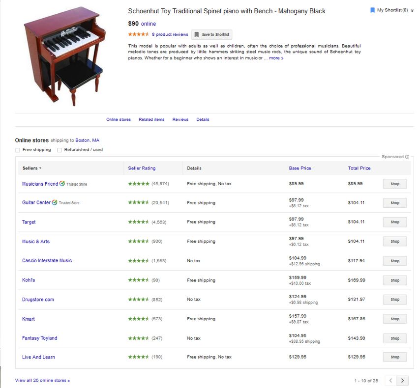
Gorodnichenko, Sheremirov, and Talavera              Price Setting in Online Markets      5

    Although e-commerce has penetrated virtually all sectors of the economy and
internet markets attracted enormous attention of economists, analyses of online prices
have been fragmented (see Ellison and Ellison 2005 for an early survey). The data used
in these studies typically cover a limited number of consumer goods in categories that
feature early adoption of e-trade, such as books and CDs (e.g., Brynjolfsson and Smith
2000), span a short period of time, usually not exceeding a year (e.g., Lünnemann and
Wintr 2011), or cover a specific seller (e.g., Einav et al. 2015). In spite of increasing
efforts to scrape more and more prices online to broaden data coverage (Cavallo and
Rigobon 2012; Cavallo 2013, 2015; Cavallo et al. 2014, 2015), we are aware of just a
handful of studies that have information on the quantity margin for internet commerce
(e.g., Chu et al. 2008; Baye et al. 2009; Soysal and Zentner 2014; Einav et al. 2015).
These studies rely on data from a particular seller and usually have limited coverage
of goods. For example, Baye et al. (2009) use data from the Yahoo! Kelkoo price
comparison site to estimate the price elasticity of clicks for 18 models of personal
digital assistants sold by 19 different retailers between September 2003 and January
2004. Einav et al. (2015) have much broader product coverage; but as they focus on
pricing that is specific to eBay, it is hard to generalize their results to other stores. In
contrast, the data used in this paper combine a broad coverage of consumer goods with
information on the number of clicks each price quote received at a daily frequency
for almost two years, a degree of data coverage that has not been within the reach
of researchers in the past. These unique properties of our data allow us to provide a
comprehensive analysis of the properties of online prices and to move beyond studying
particular segments of this market or particular pricing moments. For example, relative
to our earlier work (Gorodnichenko and Talavera 2017), we cover price dispersion and
the properties of price adjustment (frequency, size, and synchronization of sales and
of regular price changes) in much greater detail, study predictors of online prices’
properties, and utilize clicks to have a better measure of prices relevant to consumers
for a wide spectrum of goods sold online. Thus, apart from presenting new findings,
this paper validates the results found in scraped data and multichannel sellers (i.e.,
sellers with online and offline presence).
    High-quality data for online prices are not only useful to estimate price rigidity and
other properties of price adjustment in online commerce but also allow comparing the
behavior of prices online and offline. Empirical studies on price stickiness usually
document substantial price rigidity in brick-and-mortar retail stores (Klenow and
Kryvtsov 2008; Nakamura and Steinsson 2008; Klenow and Malin 2010). Theoretical
models explain it with exogenous time-dependent adjustment (Taylor 1980; Calvo
1983), menu costs (Sheshinski and Weiss 1977; Mankiw 1985), search costs for
consumers (Benabou 1988, 1992), the costs of updating information (Mankiw and
Reis 2002), or sticker costs4 (Diamond 1993). Why prices are sticky is important for
real effects of nominal shocks. For example, in the standard New Keynesian model
with staggered price adjustment, nominal shocks change relative prices and, hence,

4.   That is, the inability of firms to change the price for inventories.

Journal of the European Economic Association
Preprint prepared on September 19, 2017 using jeea.cls v1.0.
Gorodnichenko, Sheremirov, and Talavera Price Setting in Online Markets 6
affect real variables (Woodford 2003).5 On the other hand, Head et al. (2012) construct
a model with price stickiness coming from search costs that delivers monetary
neutrality. Overall, our results suggest either that standard macroeconomic models of
price rigidities, which emphasize menu costs and search costs, are likely incomplete
or that the magnitude of such costs is nontrivial in online markets, too. Since
the assumptions of popular mechanisms rationalizing imperfect price adjustment
in traditional markets do not fit well with e-commerce, more research is required
to understand sources of price rigidities and dispersion. For example, obfuscation
emphasized in Ellison and Ellison (2009) and more intensive price experimentation
(Baye et al. 2007) may provide building blocks for future theories.6
The rest of the paper is structured as follows. The data are described in the next
section. Section 3 provides estimates of the frequency, synchronization, and size
of price changes and sales and compares them to pricing moments in brick-and-
mortar stores. Section 4 examines properties of price dispersion in online markets.
This section also explores how product entry and exit are related to observed price
dispersion and other pricing moments. Section 5 looks at the variation of prices
over time, including conventional sales seasons and days of the week and month.
Concluding remarks are in Section 6.
2. Data
We use proprietary data from a leading online-shopping/price-comparison platform7
on daily prices (net of taxes and shipping costs) and clicks for more than 50,000
goods in 22 broadly-defined consumer categories in the United States and the United
Kingdom between May 2010 and February 2012. This dataset is a stratified random
sample of goods with at least one click per day obtained directly from the shopping
platform; hence, it is reliable and unlikely to have measurement error associated with
scraping price observations from the internet. The platform—and our dataset—cover
virtually all product categories available on the internet. Broad product coverage
allows us to expand our understanding of how online markets work, which up until
now has been shaped largely by data on electronics, books, or apparel. Moreover,
as a good is defined at the unique product level, similar to the Universal Product
Code (UPC), this dataset is comparable to those used in the price-stickiness literature
(e.g., scanner data) and therefore allows us to compare price setting in online and
5. In this model, price stickiness, in addition, leads to inflation persistence that is inherited from the
underlying process for the output gap or marginal cost. Modifications of this model that include shocks
to the Euler equation, the indexation of price contracts, or “rule-of-thumb” behavior give rise to intrinsic
inflation persistence; see Fuhrer (2006, 2010).
6. Other prominent theoretical models that provide possible explanations for price variation include
Bakos (1997), Baye and Morgan (2001), and Hong and Shum (2006). De los Santos et al. (2012) test
consumer search models using online browsing data.
7. Examples of major shopping platforms and price comparison websites include Google Shopping,
Nextag, and Pricegrabber. Online Appendix A describes how a typical shopping platform operates.
Journal of the European Economic Association
Preprint prepared on September 19, 2017 using jeea.cls v1.0.Gorodnichenko, Sheremirov, and Talavera Price Setting in Online Markets 7
brick-and-mortar stores. However, we cannot match individual products online and
offline, as UPC codes are masked within narrow categories. For example, we know
that product i is a particular cell phone, but we do not know its brand or model.
Having a large sample of sellers (more than 27,000), we can look at price setting
through the lens of competition between stores, analyze price dispersion across them,
and examine the effect of market characteristics on price adjustment. Despite the large
number of sellers on the platform overall, typically there are a limited number of
sellers offering a particular product, thus making it easy to search for the best price.
Next, since the data are recorded at a daily frequency, we can study properties of prices
at high frequencies. Last and foremost, information on clicks can be used to focus on
products that are relevant for online business. Shopping/price-comparison platforms
routinely use clicks as a proxy for transactions they generate for a seller’s listing, and
the service charge for using the platform is typically per-click. The rate of conversion
from clicks to purchases is about 2%–3% (CPC Strategy 2014), and generally clicks
are correlated with sales at the aggregate level. Large stores (which sell more than 100
goods in our sample) receive the lion’s share of clicks. Thus, using clicks as weights
downplays the role of small sellers.
Note that because the sample is stratified by goods rather than stores, one should
bear in mind that even “small” stores in our data can sell many goods that were not
sampled. For example, if the sample of goods is 1% of the population, a store selling
10,000 goods will be represented by only 100 randomly drawn goods. Hence, a low
number of goods per store should not be interpreted as suggesting that the stores in
the sample are small or that the sample is populated nearly exclusively by marketplace
sellers typical for eBay and other shopping platforms. While the sampling is not
appropriate for measuring the absolute size of stores, it does preserve the ranking
of stores by size and market shares.
Unfortunately, we do not have information on actual sales, local taxes, shipping
costs, detailed description of goods, names of sellers, sellers’ costs/bids/budgets, and
ratings of goods and sellers. Although the sample period is long relative to previous
studies of online markets, it is not long enough to accurately measure store entry
and exit, product turnover, or price behavior at longer horizons. Overall, we use the
most comprehensive dataset on online prices made available to researchers by a major
online shopping platform.
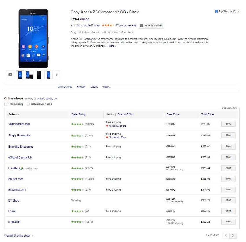
Shopping Platform. The shopping site that donated the data is a huge and growing
price comparison platform, which utilizes a fully commercialized product-ad system
and has global operational coverage (including countries such as Australia, Brazil,
China, the Czech Republic, France, Germany, Italy, Japan, the Netherlands, Spain,
Switzerland, the United Kingdom, and the United States). Information available to
consumers on the platform includes a product description and image, the number of
reviews, availability, and minimum price across all participating stores. Consumers are
also offered an option to browse other items in the same product category. Information
about sellers—name, rating, number of reviews, base price, total price with tax and
Journal of the European Economic Association
Preprint prepared on September 19, 2017 using jeea.cls v1.0.Gorodnichenko, Sheremirov, and Talavera Price Setting in Online Markets 8
shipping cost, and a link to the seller’s website—is located below the description.8 The
on-screen order of the sellers is based on their quality rank (computed using reviews,
click-through rate, etc.) and the bid price per click. Consumers can sort the sellers
by the average review score, base price, or total price. The platform also provides
information (but not the price) about nearby brick-and-mortar stores that offer the
same product.
The seller specifies devices, language, and geographical location where the ad
will appear, as well as a cost-per-click bid and maximum daily spending on the ad.
The seller may be temporarily suspended if daily spending reaches the cap or the
monthly bill is not paid on time. Remarkably, there is no explicit cost of an impression
(a listing display) or a price change. The seller pays for clicks only—although there
is an implicit cost of having a low click-through rate (number of clicks divided by
number of impressions) associated with an increase in the bid price required to reach
the same on-screen position in the future. The online platform’s rules represent both
opportunities (no direct costs) and limitations (bad reviews or low click-through rate
if unsuccessful) of price experimentation on the platform and, overall, favor dynamic
pricing. The seller’s information set consists of the number of clicks for a given period,
the number of impressions, the click-through rate, the average cost per click, the
number of conversions (specific actions, such as purchase on the seller’s website), the
cost per conversion, and the total cost of the ad—all are available through the seller’s
ad-campaign account. The shopping platform explicitly recommends that its sellers
remove ads with a click-through rate smaller than 1% in order to improve their quality
rank (which can be monetized through a lower bid price for the same on-screen rank
in the future).
Our platform and similar platforms are used by consumers intensively as these
platforms offer easy price comparison and shopping experience. For example, a study
by the European Commission (2014) reports that 74% of all shoppers in the European
Union use internet comparison tools (price comparison websites are the most popular
ones: 73% of comparison tool users) to compare prices (69% of users) and find the
cheapest price (68% of users). Forty-eight percent of users check a price comparison
website before making an online purchase, and 35% of users report that the use
of a comparison tool results in a purchase. While there is no such study for the
United States, scattered reports paint a similar picture. For example, Statista (2015), a
consultant firm, reports that 16% of U.S. consumers in 2014 used a price comparison
website to make their most recent purchase, thus making price comparison websites
the most popular location for making e-commerce purchases.
Coverage. The sample covers 52,776 goods sold across 27,308 online stores in the
United States and 52,767 goods across 8,757 stores in the United Kingdom in 2,055
narrowly defined product categories, which are aggregated into 22 broad categories
8. Gorodnichenko and Talavera (2017) document that prices reported on a price comparison website
(similar to the one used in this paper) are highly correlated with the corresponding prices quoted by online
stores (correlation is approximately 0.98). Likewise, Cavallo (2017) reports a high consistency of offline
and online prices for multichannel sellers with presence on the internet and in conventional markets.
Journal of the European Economic Association
Preprint prepared on September 19, 2017 using jeea.cls v1.0.Gorodnichenko, Sheremirov, and Talavera Price Setting in Online Markets 9
TABLE 1. Data Coverage
United States United Kingdom
Number of Number of Number of Number of
Category Goods Sellers Goods Sellers
(1) (2) (3) (4)
Media 14, 370 3, 365 14, 197 1, 136
Electronics 7, 606 8, 888 7, 693 2, 967
Home and Garden 5, 150 6, 182 5, 311 1, 931
Health and Beauty 4, 425 3, 676 4, 425 1, 362
Arts and Entertainment 2, 873 2, 779 2, 945 963
Hardware 2, 831 3, 200 2, 770 1, 042
Toys and Games 2, 777 3, 350 3, 179 1, 073
Apparel and Accessories 2, 645 2, 061 2, 761 797
Sporting Goods 2, 335 2, 781 2, 392 950
Pet Supplies 1, 106 1, 241 1, 145 295
Luggage and Bags 1, 077 1, 549 1, 037 679
Cameras and Optics 978 2, 492 978 842
Office Supplies 849 1, 408 792 651
Vehicles and Parts 575 1, 539 620 390
Software 506 1, 041 545 593
Furniture 334 1, 253 338 408
Baby and Toddler 160 654 169 301
Business and Industrial 67 324 48 116
Food, Beverages, and Tobacco 67 174 69 97
Mature 43 385 30 20
Services 26 119 50 112
Not Classified 1,976 3,465 1,273 1,039
Total 52,776 27,308 52,767 8,757
(e.g., costumes, vests, and dresses are subcategories in “Apparel and Accessories,”
while hard drives, video cards, motherboards, and processors are subcategories in
“Electronics”). Importantly, this dataset includes not only electronics, media, and
apparel (categories studied before), but also product categories that have not been
studied before, such as home and garden equipment, hardware, or vehicles. A list
of broad product categories, together with the corresponding number of sellers and
goods, is provided in Table 1. Some key results presented in this paper are available at
the category level in the online appendix.
Notation. We use pist and qist to denote the price and number of clicks,
respectively, for good i offered by seller s at time t. Time is discrete, measured with
days or weeks, and ends at T , the last day (week) observed. We denote the set of
all goods, all sellers, and all time periods as G = {1, . . . , N}, S = {1, . . . , S}, and
T = {1, . . . , T }, respectively, with N being the number of goods in the dataset and
S the number of sellers. Subscripts i and s indicate a subset (or its cardinality) that
corresponds to a given good or seller. For instance, Ns ≤ N is the number and Gs ⊆ G
is the set of all goods sold by seller s, while Si ≤ S is the number and Si ⊆ S is the
set of all sellers that offer good i. We denote averages with a bar and sums with a
corresponding capital letter (e.g., p̄is = ∑t pist /T is the average price charged by seller
Journal of the European Economic Association
Preprint prepared on September 19, 2017 using jeea.cls v1.0.Gorodnichenko, Sheremirov, and Talavera Price Setting in Online Markets 10
s for good i over the entire sample period and Qit = ∑s∈S qist is the total number of
clicks that good i received across all sellers in week t).
Aggregation. We use the number of clicks as a proxy for sales, at least partially
bridging the gap between the studies of online markets, which do not have such
information, and brick-and-mortar stores, which use quantity or sales weights to
aggregate over products.9 We find that a relatively small number of products and
sellers obtain a disproportionately large number of clicks. To emphasize the difference
between price-setting properties for all products and sellers (available for scraping)
and those that actually generate some activity on the user side, we employ three
different weighting schemes to aggregate the frequency, size, and synchronization of
price changes, as well as cross-sectional price dispersion, over goods and sellers. First,
we compute the raw average, with no weights used. Second, we use click weights to
aggregate across sellers of the same product but then compute the raw average over
products. We refer to this scheme as within-good weighting. Third, we use clicks to
aggregate across both sellers and products (referred to as between-good weighting).
More specifically, let fis be, for example, the frequency of price changes for good i
offered by seller s, and Qis the total number of clicks. The three aggregate measures
(denoted by f¯, f¯w , and f¯b , respectively) are computed as follows:
1 1
f¯ = ∑ ∑ fis ,
i N s S
1 Qis
f¯w = ∑ ∑ fis · , (1)
i N s ∑s Qis
| {z }
within-good
weights
∑ Qis Qis
f¯b = ∑ s · ∑ fis · .
i |∑i ∑ Q ∑ Q
{zs is} s | s{z is}
between-good within-good
weights weights
Empirically, the difference between f¯ and f¯w is often much smaller than the
difference between either of them and f¯b , as many products have only one seller.
However, the within-good weighting appears more important if we look only at
products with a sufficiently large number of sellers. We use f¯b as our baseline click-
weighted measure, since it is the closest among the three to the corresponding brick-
and-mortar measure and incorporates information on the relative importance of goods
in the consumption basket of online shoppers. We relegate all relevant results obtained
using within-good weights f¯w to Online Appendix C.
Price Distribution and Clicks. Table 2 reports percentiles of the distribution over
goods of the average price for a good, p̄i , together with the mean and the standard
deviation of the average log price, log pi . The median good in the sample costs around
$25 in the United States and £19 in the United Kingdom. About a quarter of goods
9. Details on data aggregation from daily to a weekly frequency is relegated to Online Appendix B.
Journal of the European Economic Association
Preprint prepared on September 19, 2017 using jeea.cls v1.0.Gorodnichenko, Sheremirov, and Talavera Price Setting in Online Markets 11
TABLE 2. Distribution of Prices, local currency
Mean Log Price Mean Price, percentile
Mean SD 5 25 50 75 95 N
(1) (2) (3) (4) (5) (6) (7) (8)
Panel A: United States
No weights 3.37 1.53 4 11 25 71 474
52,776
Click weighted 4.15 1.51 7 22 61 192 852
Panel B: United Kingdom
No weights 3.13 1.56 3 8 19 57 381
52,767
Click weighted 3.82 1.44 5 17 48 134 473
Note: Columns (1)–(2) show moments of the distribution of the average (for a good) log price, log pi , columns
(3)–(7) of the average price, p̄i , and column (8) the total number of goods, N.
Panel A: United States, price distribution Panel B: United Kingdom, price distribution
5 6
No weights No weights
Click weighted Click weighted
5
4
4
3
Density
Density
3
2
2
1
1
0-.4 -.3 -.2 -.1 0 .1 .2 .3 .4 0-.4 -.3 -.2 -.1 0 .1 .2 .3 .4
Log deviation from the median-seller price Log deviation from the median-seller price
Panel C: United States, clicks vs. price Panel D: United Kingdom, clicks vs. price
.2 .2
Clicks, log deviation from median seller
Clicks, log deviation from median seller
Lowess smoothing Lowess smoothing
.1
.1
0
0
-.1
-.1-.4 -.3 -.2 -.1 0 .1 .2 .3 .4 -.4 -.3 -.2 -.1 0 .1 .2 .3 .4
Log deviation from the median-seller price Log deviation from the median-seller price
0.05 0.05
F IGURE 1. Prices and Clicks: In the top two panels, the dashed line shows the distribution of the
log price deviation from the median across sellers, and the solid line shows the between-good click-
weighted distribution of that deviation. In the bottom two panels, the dots represent data points
averaged within bins based on percentiles of the log-deviation of price. The Lowess smoothing is
calculated with a 0.05 bandwidth.
cost $11 or less; products that cost $100 or more represent around 20% of the sample.
Goods that obtain more clicks tend to be more expensive: the median price computed
using the between-good weights is $61 and £48 in the United States and the United
Kingdom, respectively.
Journal of the European Economic Association
Preprint prepared on September 19, 2017 using jeea.cls v1.0.Gorodnichenko, Sheremirov, and Talavera Price Setting in Online Markets 12
To illustrate the importance of clicks for measuring prices effectively paid by
consumers, for each good we compute the average (over time) log deviation of the
price of seller s, pist , from the median price across sellers, peit :
1
ρ̄is = ∑ log (pist / peit ) . (2)
T t
Panels A and B of Figure 1 plot the density of deviations without weights and with
the between-good weights based on the number of clicks, Qit . Applying the weights
shifts the distribution to the left by approximately 10%; that is, sellers with a price
substantially below the median product price receive a larger number of clicks.
To show the relationship between prices and clicks, Panels C and D of Figure 1
plot clicks against prices, measured as log-deviation from the median seller for a
good on a given date. To enhance visibility, we show the scatterplot for bins based
on the percentiles of the price measure, and then pass a Lowess smoother to allow
for nonlinearities in the clicks–price relationship. The figure paints a clear picture
that sellers with a price significantly below the median obtain more clicks. The curve
is flatter in the region of a positive price deviation, supporting the notion that the
clicks are especially sensitive to prices when prices are in the lower end of the price
distribution.
3. Price Stickiness
Price-adjustment frictions should be smaller for online stores than for brick-and-
mortar stores. For example, changing the price does not require printing a new
price tag and is therefore less costly. Price adjustment for online markets may also
employ algorithmic approaches (“dynamic pricing”) to avoid costs associated with
collecting and processing information as well as costs related to making collective
decisions (e.g., “meeting” costs). In a similar spirit, consumers can compare prices
across retailers without leaving their desks (smaller search costs). As a result, we
should observe a slightly higher frequency and smaller size of price changes in online
markets. At the same time, lower costs of monitoring competitors’ prices should
lead to a higher synchronization of price changes across sellers and across goods,
thus diminishing nominal non-neutrality. This section challenges these conjectures by
showing that online markets are not that different from their conventional counterparts
after all.
3.1. Regular and Posted Prices
Previous work (see Klenow and Malin 2010 for an overview) emphasizes the
importance of temporary price cuts (“sale prices”) for measuring the degree of price
rigidities. However, Eichenbaum et al. (2011) point out that sale prices carry little
weight at the aggregate level because they likely represent a reaction to idiosyncratic
Journal of the European Economic Association
Preprint prepared on September 19, 2017 using jeea.cls v1.0.Gorodnichenko, Sheremirov, and Talavera Price Setting in Online Markets 13
shocks. Hence, we make a distinction between posted prices (i.e., prices we observe
in the data) and regular prices (i.e., prices that exclude sales).
In contrast to scanner data, our dataset does not have sales flags and therefore
we use filters as in Nakamura and Steinsson (2008), Eichenbaum et al. (2011), and
Kehoe and Midrigan (2015) to identify temporary price changes.10 We consider a
price change to be temporary if the price returns to its original level within one or
two weeks. As the dataset contains missing values, we identify sales with and without
imputation, using a standard procedure in the literature.
Consider the following price series: {$2, n.a., $2, n.a., $1, $2}, where “n.a.”
denotes missing values. In the “no imputation” case, we assume that “n.a.” breaks
a price series so that we have only one series of consecutive observations, {$1, $2}. In
this case, there is one “regular” price change from $1 to $2 because $1 is preceded by
“n.a.” and not by $2. In the “imputation” case, we replace “n.a.” with an actual price if
the prices before and after “n.a.” are equal to each other. We also identify an episode as
a sale if the first observable price before “n.a.” and the last observable price after “n.a.”
are the same. That is, in our example, we replace the first “n.a.” with a $2 price and we
drop the second “n.a.” from the identification of sales. The imputed series of regular
prices thus becomes {$2, $2, $2, n.a., n.a. $2}; the imputed series of sale flags is {0,
n.a., 0, n.a., 1, 0}; and the imputed series of regular price changes is {n.a., 0, 0, n.a.,
n.a., 0}, where the first “n.a.” is due to spell truncation.11 We report statistics for the
two assumptions separately and present additional results for alternative imputation
procedures in Online Appendix Table G.2. We find that reasonable modifications to
our imputation procedure do not alter our conclusions.
Table 3 reports the frequency and size of sales. In the United States, the mean
weekly frequency of sales (columns 1 and 5), without weights, is in the range
of 1.3%–2.2%, depending on the filter. This weekly frequency is comparable to
the frequency of sales reported for prices in regular stores. There is substantial
heterogeneity in the frequency across products: we do not find sales in more than a
half of the products (see column 3). When we focus on goods that receive more clicks
(use between-good weights), sales occur more often: the mean frequency is 1.7%–
2.7% depending on a computation technique. The median size of sales is 10.5%–
11.9% with equal weights and 4.4%–5.3% with between-good weights. These sizes
are smaller than the size of sales in regular stores (about 20%–30%). Using our
10. We use both ∨- and ∧-shaped filters to account not only for temporary price cuts but also for
temporary price increases (e.g., due to stockout).
11. In this example, our “imputation” filter applies to one missing value between two observed prices. In
practice, our filters are applied up to five missing values between any two observed prices. This procedure
is valid because we compute the frequency of price changes and then use it to infer the implied duration
of price spells, instead of computing duration directly. Hence, we make no additional assumptions on
unobserved prices. We do not use imputation as our baseline frequency statistic or for any other measure
reported in this paper. Online Appendix Table G.1 shows that imputing an arbitrarily large number of
missing values between two observed prices has little effect on the frequency of price changes. To assess
the extent of imputation, Online Appendix Figure G.1 reports the distribution over goods of the share of
imputed price changes. On average, 27.3% of price changes in the U.S. sample are imputed.
Journal of the European Economic Association
Preprint prepared on September 19, 2017 using jeea.cls v1.0.Gorodnichenko, Sheremirov, and Talavera Price Setting in Online Markets 14
TABLE 3. Frequency and Size of Sales
One-Week Filter Two-Week Filter
Mean Std. Med. Med. Mean Std. Med. Med.
Freq. Dev. Freq. Size Freq. Dev. Freq. Size N
(1) (2) (3) (4) (5) (6) (7) (8) (9)
Panel A: United States
No Imputation
No weights 1.3 3.1 0.0 10.5 1.9 3.9 0.0 10.5 10, 567
Click weighted 1.7 1.9 1.4 4.4 2.6 2.5 2.2 4.8 10, 567
With Imputation
No weights 1.6 3.5 0.0 11.9 2.2 4.2 0.0 11.9 21, 452
Click weighted 1.9 1.9 1.6 4.7 2.7 2.4 2.4 5.3 21, 452
Offline Stores 1.9 n.a. n.a. 29.5
Panel B: United Kingdom
No Imputation
No weights 0.9 2.9 0.0 5.7 1.3 3.7 0.0 5.7 4, 464
Click weighted 1.3 1.7 1.0 2.5 1.8 2.3 1.4 2.9 4, 464
With Imputation
No weights 1.1 3.3 0.0 6.2 1.6 4.0 0.0 5.9 10, 754
Click weighted 1.4 1.8 1.0 2.5 2.0 2.4 1.5 3.2 10, 754
Offline Stores 0.3 n.a. n.a. 7.0
Notes: Column (1) reports the average weekly frequency of sales across goods (%), column (2) the standard
deviation of the frequency across goods, column (3) the frequency for the median good, and column (4) the
absolute size of sales for the median good measured by the log difference between the sale and regular price
(multiplied by 100). In all the four columns, we identify sales using the one-week, two-side sale filter (see the
text). Columns (5)–(8) report the same statistics for the two-week sale filter. Column (9) reports the number
of goods. The statistics for offline stores are from Nakamura and Steinsson (2008) for the United States and
Kryvtsov and Vincent (2014) for the United Kingdom; the mean frequency is converted to the weekly rate.
“imputation” procedure for missing values tends to generate a higher frequency and
size of sales. The magnitudes are similar for the United Kingdom, although there is
some variation across countries for disaggregate categories of goods, which likely
reflects idiosyncratic factors affecting specific markets in the two countries.
We also report the degree of synchronization of sales (across sellers for a given
good or across goods within a given seller), which can be informative about the nature
of sales.12 For example, sales could be strategic substitutes (low synchronization)
or complements (high synchronization), they could be determined by seller-specific
factors (low synchronization) or aggregate shocks (high synchronization).13 We find
(Online Appendix Table G.3) that the synchronization of sales across sellers is below
2% in each country. The synchronization of sales across goods within a seller is
12. We define the sale synchronization rate as the mean share of sellers that put a particular product on
sale when another seller of the same good has a sale. In particular, if B is the number of sellers of good i
and A of them have sales, the synchronization rate is computed as (A − 1) /(B − 1); that is, the statistic is
calculated only conditional on having at least one sale. See Section 3.4 for more details.
13. Guimaraes and Sheedy (2011) propose a model of sales that are strategic substitutes. Alternatively,
Anderson et al. (2017) present evidence that sales are largely determined by seller-specific factors and best
described as being on “autopilot” (not related to aggregate variables and not synchronized).
Journal of the European Economic Association
Preprint prepared on September 19, 2017 using jeea.cls v1.0.Gorodnichenko, Sheremirov, and Talavera Price Setting in Online Markets 15
less than 3% in the United States and 4% in the United Kingdom. Because the
degree of synchronization is similar to the frequency of sales, we conclude that the
synchronization of sales is low.
3.2. Frequency and Size of Price Changes
Frequency. We compute the frequency of price adjustment per quote line as the
number of nonzero price changes divided by the number of observed price changes.14
This measure is then aggregated to the good level. Based on the frequency of price
adjustment, we also compute the implied duration of price spells under the assumption
of constant hazards. Specifically, let ϕist = I{qis,t > 0}I{qis,t−1 > 0} be the indicator
function whether a price change (either zero or not) is observed, Πis = ∑t ϕist the
number of observed price changes per quote line, and χist = I{|∆log pist | > 0.001} the
indicator function for a nonzero price change. Then, the frequency of price adjustment
per quote line is the number of nonzero price changes divided by the number of
observed price changes,
∑ χist
fis = t . (3)
Πis
We aggregate this measure to the good level by taking the raw, f¯i , and click-weighted,
f¯iw , average across quote lines with at least five observations for a price change:
1
f¯i = ∑ fis I {Πis > 4} , (4)
∑s∈Si I{Πis > 4} s∈Si
ϕ
∑ fis I {Πis > 4}Qis
f¯iw = s ϕ , (5)
∑s I{Πis > 4}Qis
ϕ
where Qis = ∑t qist ϕist . The former measure is referred to as “no weights” and
the latter as “within-good weights.” The “between-good” measure reports the
distribution across goods of f¯iw with Wi = QΠ Π
i / ∑i∈G Qi used as weights, where
Π ϕ
Qi = ∑s∈Si I{Πis > 4}Qis . The implied duration of price spells is then computed as
1
d¯i = − . (6)
ln 1 − f¯i
The first two rows in each panel of Table 4 show the estimated frequency of price
changes and the corresponding implied duration. In the United States, the median
implied duration of price spells varies from 7 to 12 weeks when no weights are applied
and from 5 to 6 weeks when we use weights across sellers and goods. When we
apply the one-week sale filter, the duration of price spells increases by 20%–65%.
14. This measure is analogous to the one used by Bils and Klenow (2004), Klenow and Kryvtsov (2008),
and Nakamura and Steinsson (2008). In line with Eichenbaum et al. (2011), price changes smaller than
0.1% are not counted as price changes. We exclude quote lines with fewer than five observations. Following
Nakamura and Steinsson (2008), we compute the frequency of price changes and then infer the implied
duration of spells, to avoid bias due to spell truncation.
Journal of the European Economic Association
Preprint prepared on September 19, 2017 using jeea.cls v1.0.Gorodnichenko, Sheremirov, and Talavera Price Setting in Online Markets 16
TABLE 4. Frequency and Size of Price Changes
No Imputation With Imputation
No Click No Click Offline
Weights Weighted Weights Weighted Stores
(1) (2) (3) (4) (5)
Panel A: United States
Posted Price
Median frequency, % 14.0 19.3 8.2 15.7 4.7
Implied duration, weeks 6.6 4.7 11.6 5.8 20.8
Median absolute size, log points 11.0 11.2 10.7
Regular Price
Median frequency, % 8.8 14.5 7.0 12.9 2.1
Implied duration, weeks 10.9 6.4 13.9 7.3 47.1
Median absolute size, log points 10.9 10.9 8.5
Panel B: United Kingdom
Posted Price
Median frequency, % 12.8 20.0 7.7 16.3 4.6
Implied duration, weeks 7.3 4.5 12.5 5.6 21.2
Median absolute size, log points 5.1 8.5 11.1
Regular Price
Median frequency, % 7.7 15.8 6.7 14.3 3.2
Implied duration, weeks 12.5 5.8 14.5 6.5 30.7
Median absolute size, log points 5.0 7.6 8.7
Notes: Column (1) reports the frequency and size of price changes when missing values are dropped and no
weights are applied. Column (2) reports click-weighted results using our default weighting method. Columns
(3)–(4) report the analogous statistics when missing values are imputed (if the next available observation is
within four weeks and there is no price change). Column (5) shows the corresponding statistics from Nakamura
and Steinsson (2008) for the United States and Kryvtsov and Vincent (2014) for the United Kingdom, converted
to a weekly frequency. Regular prices are identified using a one-week filter for sales.
The magnitudes are similar for the United Kingdom. We also find that the frequency
of price increases is approximately equal to the frequency of price decreases (Online
Appendix Table G.4). Despite significant heterogeneity in the frequency of price
changes across products (Online Appendix D), our aggregate statistics are not driven
by any particular categories (Online Appendix E).
Price spells for online stores appear significantly shorter than for brick-and-mortar
stores (by up to a half for posted prices and by two-thirds for regular prices). However,
with spells of up to four months, online prices are far from being completely flexible,
pointing toward price-adjustment frictions other than the conventional nominal costs
of price change. At the same time, goods that receive a large number of clicks have
more flexible prices—with the average duration of only 5–7 weeks for regular and
posted prices. These magnitudes are similar to the results reported in earlier papers
(Lünnemann and Wintr 2011; Boivin et al. 2012; Gorodnichenko and Talavera 2017)
for specific segments of e-commerce.15 We find the same pattern when we compare
15. The frequency of price adjustment in our data is higher than the frequency of price adjustment for
multichannel stores (Cavallo 2017). The adjustment of online prices for this type of stores is likely “slowed
Journal of the European Economic Association
Preprint prepared on September 19, 2017 using jeea.cls v1.0.Gorodnichenko, Sheremirov, and Talavera Price Setting in Online Markets 17
the properties of online and offline prices within narrowly defined product categories
(see Online Appendix F). Therefore, our findings are not driven by differences in
the composition of goods in e-commerce and conventional retailers.16 Because large
online stores receive a large share of clicks (Online Appendix Figure G.2), our results
with between-good weights (our baseline) are similar to the results we obtain for the
sample restricted to large stores (Online Appendix Table G.5). However, when we
focus on very large stores (100+ products), we find smaller shares of stores that do not
change their prices at all (Online Appendix Figure G.3). We also find that the hazard of
price adjustment is decreasing in the duration of price spells (Online Appendix Figure
G.4).
Size. Using our notation in the previous section, we can write the average absolute
size of price changes for good i as follows:
1
|∆log pi | = ∑ ∑ |∆log pist | ·χ ist . (7)
∑s∈Si ∑t χist s∈Si t
χ
Next, let Qi = ∑s∈Si ∑t qist χist be the total number of clicks when a nonzero price
change occurs. The within-good weighted average of this measure can be written as
w qist χist
|∆log pi | = ∑∑ χ |∆log pist | . (8)
s∈Si t Q
| {zi }
within-good
weights
Finally, the between-good weighted results are based on the weighted distribution of
w χ χ
|∆log pi | with weights Wi = Qi / ∑i∈G Qi , implemented in a similar fashion as for the
frequency of price adjustment.
The last row of each panel in Table 4 reports the absolute size of price change.
In the United States, online sellers change their prices on average by 11%, which
is somewhat larger than the estimates reported in earlier studies. This magnitude is
remarkably stable and close to that for brick-and-mortar stores. Again, we find similar
results when we compare the size of price changes for online and offline prices for
goods within narrowly defined product categories. The fact that online sellers adjust
their prices more often than their offline counterparts, but by roughly the same amount,
indicates the presence of implementation costs of price change. Incidentally, regular
and temporary changes are approximately of the same size. In the United Kingdom,
the size of price changes is smaller (approximately 5%), but it approaches the U.S.
down” by the stickiness of offline prices and the apparent desire of these stores to maintain consistency of
online and offline prices.
16. Ideally, one would like to match specific goods sold online to exactly the same goods sold offline,
thereby completely eliminating potential differences in the composition. Unfortunately, we cannot do this
because we do not have names or detailed descriptions of the goods in our dataset, and available offline-
price datasets with broad coverage (e.g., BLS micro-level price data) do not have detailed descriptions of
goods.
Journal of the European Economic Association
Preprint prepared on September 19, 2017 using jeea.cls v1.0.Gorodnichenko, Sheremirov, and Talavera Price Setting in Online Markets 18
statistic when between-good weights are applied (8.5%). Price decreases are slightly
smaller than price increases (Online Appendix Table G.6). We also find that very large
stores (100+ products) are less likely than small stores to have large price changes
(Online Appendix Figure G.5).
3.3. Do Prices Change Mostly during Product Replacement?
Nakamura and Steinsson (2012) emphasize that product replacement is potentially
an important margin of price adjustment and that focusing on goods with short
product lives and no price changes can overstate the degree of price rigidity (“product
replacement bias”). In the context of online prices, (Cavallo et al. 2014, henceforth,
CNR) scraped price data from selected online retailers (Apple, H&M, IKEA, and
Zara) and documented three facts related to the product replacement bias: (1) most
products do not change their prices throughout the lifetime (77% in the U.S. sample);
(2) the median duration of product life is short (15 weeks); and (3) products that live
longer are more likely to have at least one price change (a product observed for more
than two years is 39 percentage points more likely than an average product to have at
least one price change).
To assess the importance of product replacement for measurement of price
rigidities in online markets, we first compute the share of products with a constant
price over their lives and compare these products to products with at least one price
change.17 In the United States, 11.9% of goods have a constant price within their life
span (column 1 of Table 5)—this is significantly lower than 77% in CNR. Moreover,
goods with no price change account for only 1% of total clicks. When we look at
products in apparel that are offered by one seller only (hence, a sample of goods that is
more similar to those in H&M or Zara), the share of goods with no price changes rises
to 31% and the corresponding share of clicks to 26% (column 3). When we further
remove jewelry and watches, which represent a large share of apparel and accessories
in our data but are not key for H&M and Zara, the magnitudes further increase to
42% and 31%, respectively (column 5). We observe a similar pattern in the United
Kingdom. Hence, the prevalence of goods with no price changes in the CNR data
appears to be determined by their sample of goods and sellers.
In the next step, we compare (Table 5) goods with and without price changes
along four dimensions: (1) the average number of clicks for a price quote; (2) the
observed duration of product life; (3) the number of price quotes with a click; and (4)
the number of sellers. While these two groups of goods are similar in terms of (1),
we see considerable differences in all other dimensions. In the United States, goods
with at least one price change, on average, span over 57 weeks, have 12 price quotes,
17. Our data do not provide direct information about when a good is introduced or discontinued. We
approximate entry and exit of goods with the dates when goods appear for the first and last time. We also
drop products that enter or exit within the first or last five weeks of our data to avoid truncation bias in
product-life duration. We find similar results when we exclude goods with truncated entry/exit (Online
Appendix Table G.7).
Journal of the European Economic Association
Preprint prepared on September 19, 2017 using jeea.cls v1.0.You can also read