Pulsational properties of ten new slowly pulsating B stars
←
→
Page content transcription
If your browser does not render page correctly, please read the page content below
A&A 633, A122 (2020)
https://doi.org/10.1051/0004-6361/201935478                                                                          Astronomy
c ESO 2020                                                                                                            &
                                                                                                                     Astrophysics

           Pulsational properties of ten new slowly pulsating B stars
                        M. Fedurco1 , E. Paunzen2 , S. Hümmerich3,4 , K. Bernhard3,4 , and Š. Parimucha1

      1
          Institute of Physics, Faculty of Science, P. J. Šafárik University, Park Angelinum 9, Košice 040 01, Slovak Republic
          e-mail: miroslav.fedurco@student.upjs.sk
      2
          Department of Theoretical Physics and Astrophysics, Masaryk University, Kotlářská 2, 611 37 Brno, Czech Republic
      3
          American Association of Variable Star Observers (AAVSO), 49 Bay State Rd., Cambridge, MA 02138, USA
      4
          Bundesdeutsche Arbeitsgemeinschaft für Veränderliche Sterne e.V. (BAV), 12169 Berlin, Germany

      Received 15 March 2019 / Accepted 5 December 2019

                                                                   ABSTRACT

      Context. Slowly pulsating B (SPB) stars are upper main-sequence multi-periodic pulsators that show non-radial g-mode oscillations
      driven by the κ mechanism acting on the iron bump. These multi-periodic pulsators have great asteroseismic potential and can be
      employed for the calibration of stellar structure and evolution models of massive stars.
      Aims. We collected a sample of ten hitherto unidentified SPB stars with the aim of describing their pulsational properties and identi-
      fying pulsational modes.
      Methods. Photometric time series data from various surveys were collected and analyzed using diverse frequency search algorithms.
      We calculated astrophysical parameters and investigated the location of our sample stars in the log T eff vs. log L/L diagram. Current
      pulsational models were calculated and used for the identification of pulsational modes in our sample stars. An extensive grid of
      stellar models along with their g-mode eigenfrequencies was calculated and subsequently cross-matched with the observed pulsa-
      tional frequencies. The best-fit models were then used in an attempt to constrain stellar parameters such as mass, age, metallicity, and
      convective overshoot.
      Results. We present detected frequencies, corresponding g-mode identifications, and the masses and ages of the stellar models pro-
      ducing the best frequency cross-matches. We partially succeeded in constraining stellar parameters, in particular concerning mass
      and age. Where applicable, rotation periods have been derived from the spacing of triplet component frequencies. No evolved SPB
      stars are present in our sample. We identify two candidate high-metallicity objects (HD 86424 and HD 163285), one young SPB star
      (HD 36999), and two candidate young SPB stars (HD 61712 and HD 61076).
      Conclusions. We demonstrate the feasibility of using ground-based observations to perform basic asteroseismological analyses of
      SPB stars. Our results significantly enlarge the sample of known SPB stars with reliable pulsational mode identifications, which pro-
      vides important input parameters for modeling attempts aiming to investigate the internal processes at work in upper main-sequence
      stars.

      Key words. asteroseismology – stars: early-type – stars: variables: general

1. Introduction                                                            rotation, on the lifetime of a star. Asteroseismic analyses of SPB
                                                                           stars are therefore expected to contribute to the calibration of
Slowly pulsating B (SPB) stars were first described as a class by          stellar structure and evolution models of massive stars, for which
Waelkens (1991). They are main-sequence (MS) stars of spectral             the observed mass distribution significantly contradicts theoret-
types B2 to B9 (i.e., 22 000–11 000 K), which show non-radial              ical predictions (Castro et al. 2014). In addition, these analyses
g-mode oscillations driven by the κ mechanism acting on the                can be employed to determine and calibrate internal parameters
iron bump (Gautschy & Saio 1993). These SPB stars are multi-               such as the convective overshoot parameter or envelope mixing
periodic pulsators whose observed periods range from 0.3 d to              (Moravveji et al. 2015, 2016), which are not directly observable
about 5 d (De Cat 2007).                                                   but have a significant influence on stellar structure and evolution
    Several fast-rotating SPB stars have been described; the               (Pápics et al. 2015; Buysschaert et al. 2018). Furthermore, non-
majority, however, seem to be comparably slow rotators (De Cat             rigid rotational profiles can be studied by determining the spac-
2007; Degroote et al. 2011). There also exist very slowly rotat-           ing between rotationally split modes (Pápics et al. 2017; Triana
ing SPB stars like KIC 10526294 (rotation period of about 188 d;           et al. 2015).
Pápics et al. 2014). This is remarkable as the mean projected rota-             Current asteroseismic modeling attempts are mainly based
tional velocity (υ sin i) of B-type stars well exceeds 100 km s−1          on quasi-uninterrupted observational data from space telescopes
(Abt et al. 2002), which induces strong meridional circulation             such as Convection, Rotation and planetary Transit (CoRoT)
and mass loss (Dolginov & Urpin 1983).                                     (Auvergne et al. 2009) or Kepler (Borucki 2016) because their
    Stars of the upper MS are characterized by a convective core           continuity and precision enable reliable mode identification and
and a radiative envelope. The asteroseismic potential of SPB               help to constrain basic stellar parameters such as mass, luminos-
stars has been recognized early on (De Cat 2007). These stars              ity, and effective temperature with great precision (Szewczuk &
are perfect test laboratories of ill-understood processes that have        Daszyńska-Daszkiewicz 2018). However, owing to their long-
a significant influences, such as diffusion and internal differential      period, gravity-driven oscillations, SPB stars lend themselves

                                                        Article published by EDP Sciences                                        A122, page 1 of 11
A&A 633, A122 (2020)
perfectly for asteroseismic modeling using ground-based survey et al. 1997), Optical Monitoring Camera (OMC; Alfonso-Garzón
data with rather low cadence. et al. 2015), and Wide Angle Search for Planets (SuperWASP;
Pulsation in pre-MS (PMS) stars is of special interest as it Street et al. 2003). In this way, a sample of ten newly iden-
allows the investigation of the short-lived early phases of stel- tified SPB variables boasting extensive time series photometry
lar evolution with oscillations (Zwintz et al. 2015), thereby pro- was collected (cf. Table 1).
viding valuable constraints and input parameters for theoreti- HD 48497, HD 61076, HD 61712, HD 86424, HD 115067,
cal considerations. Dedicated effort has led to the discovery of HD 163285, and HD 168121 were first reported as variables on
γ Doradus and, in particular, δ Scuti pulsation in PMS objects the basis of Hipparcos data (ESA 1997; Koen & Eyer 2002).
(e.g., Zwintz et al. 2013; Ripepi et al. 2015), but the situa- Nichols et al. (2010) report the variability of HD 66181 using
tion is less clear for SPB stars. Gruber et al. (2012) identify the pointing control camera of the Chandra X-ray Observa-
two SPB stars in the vicinity of the young open star cluster tory. However, all these stars lack deeper studies and their vari-
NGC 2244; however, the available proper motion and radial ability types have not been determined. Consequently, the stars
velocity data were insufficient to confirm their cluster mem- are listed as variable stars of unspecified type (type VAR) in
bership. Zwintz et al. (2009) discovered ten SPB variables in the VSX. HD 36999 and HD 97895 are listed as suspected vari-
the field of NGC 2264, another young open cluster. Later on, able stars in the GCVS and VSX.
Zwintz et al. (2017) investigate four SPB variables belonging
to NGC 2264 in detail. Interestingly, despite the derived ages
2.2. Photometric data reduction and analysis
between one and six million years, the authors find that all stars
seem to be early zero age MS (ZAMS) objects that have already Only data from the third phase of the All Sky Automated Survey
left the PMS phase. The search for PMS SPB pulsators, there- project (ASAS-3) were taken into account; measurements with
fore, has not yielded any conclusive results yet, and identifying quality assignments “C” and “D” were excluded. Mean V mag-
suitable candidates remains of special interest. nitudes were calculated as the weighted average of the values
In this paper, we present photometric time series analysis provided in the five different apertures available. To check the
of ten newly identified SPB stars together with an asteroseis- feasibility of this approach, we subsequently restricted our anal-
mic analysis aimed at the identification of pulsational modes. ysis to the “best” aperture as indicated by the ASAS-3 system for
These results significantly add to our knowledge of the pulsa- any given star. No significant differences were found between the
tional properties of these stars and allow us to constrain astro- two approaches. Finally, a basic 5σ clipping was performed to
physical parameters, which helps to throw more light on the clean the light curves from outliers.
internal processes at work in upper MS stars. The ASAS-SN measurements are taken with different cam-
eras, which we treated separately. The mean for each individual
data set was calculated, and data points were deleted on a 5σ
2. Target selection, photometric data sources, basis. After that, the data of the individual cameras were merged.
reduction, and analysis In the case of Hipparcos and OMC data, a 5σ clipping algo-
rithm was applied.
The following sections give details on the sample selection, the Measurements with an error larger than 0.05 mag were
employed photometric time series data, and our methods of anal- excluded from the SuperWASP data sets. Each camera was
ysis. treated separately and the mean for each individual data set was
derived; data points were deleted on a 5σ basis. The data of the
individual cameras were then merged. Applying this procedure
2.1. Target selection and data sources
also corrects for the different offsets of the cameras. However,
For the sample selection, we resorted to The International Vari- for larger data sets, we also separately investigated the measure-
able Star Index (VSX; Watson et al. 2006), which is the most ments from each camera.
up-to-date and accurate variable star database available. To iden- The resulting light curves were examined in more detail
tify new SPB stars, we systematically investigated suspected and using the program package PERIOD04 (Lenz & Breger 2005),
known variable stars with periods typical for SPB stars and a which performs a discrete Fourier transform. An iterative pre-
spectral type of B or A. The extension to spectral type A was whitening procedure was used to extract all significant fre-
deemed necessary to identify objects that had been spectroscop- quencies with a signal-to-noise ratio above 4. The results from
ically misclassified. PERIOD04 were checked with the CLEANEST and phase dis-
In the given spectral type range on the MS, SPB stars persion minimization (PDM) algorithms as implemented in the
coexist with other types of photometric variables such as Be program package PERANSO (Paunzen & Vanmunster 2016).
stars (Rivinius et al. 2013) and rotationally variable CP2/4 stars The same results were obtained within the derived errors, which
(Preston 1974). While Be stars usually exhibit complex variabil- depend on the time series characteristics, i.e., the distribution
ity on timescales ranging from a few minutes to decades, the of measurements over time and the photon noise. All signif-
latter objects, which are also known as α2 Canum Venaticorum icant frequencies are listed in Table 2. Amplitude spectra and
(ACV) variables (Samus et al. 2017), exhibit surface abundance residuals, as derived with PERIOD04, are given in the appendix
patches or spots and variability periods in the same range as (Fig. A.1).
SPB stars. Their variability, however, is strictly monoperiodic
(Netopil et al. 2017) and can therefore be easily distinguished 3. Log T eff vs. log L/L diagram
from SPB type pulsation.
After the collection of an initial sample list, we searched To check whether our sample stars fall within the regime
for the availability of photometric observations in the databases of known SPB stars, we collected a control sample of well-
of the following surveys: All Sky Automated Survey (ASAS; established SPB variables (i.e., stars with a detailed astero-
Pigulski 2014), All-Sky Automated Survey for Supernovae seismic analysis available) that also boast uvbyβ photometry
(ASAS-SN; Kochanek et al. 2017), Hipparcos (van Leeuwen (Paunzen 2015). We gleaned the BV magnitudes from the
A122, page 2 of 11M. Fedurco et al.: Pulsational properties of ten new slowly pulsating B stars
Table 1. Astrophysical parameters of our sample stars.
HD HIP/TYC Spec. type T eff log g Parallax AV V MV BC log L/L
(K) (mas) (mag) (mag) (mag) (mag)
36999 4778-1364-1 B7 V 13 700 4.31 2.53(7) 0.20(5) 8.470(21) +0.28(8) −1.02 2.20(3)
48497 32221 B5 V 14 550 4.32 2.96(6) 0.13(4) 7.513(8) −0.26(6) −1.17 2.47(2)
61076 36938 B5/7 III 14 900 4.42 2.15(3) 0.39(8) 9.130(17) +0.40(9) −1.23 2.23(4)
61712 37222 B7/8 V 13 900 4.28 2.00(4) 0.23(10) 8.961(14) +0.24(11) −1.05 2.23(4)
66181 6558-2365-1 B5 V 15 450 4.35 1.93(12) 0.26(7) 7.447(7) −1.39(15) −1.32 2.98(6)
86424 48811 B9 V 12 850 4.47 1.76(4) 0.30(5) 9.298(14) +0.23(7) −0.86 2.15(3)
97895 54970 B4 V 15 050 4.39 1.44(7) 0.32(16) 8.755(12) −0.77(19) −1.26 2.71(8)
115067 64658 B8 V 13 650 4.17 1.92(9) 0.19(11) 8.062(12) −0.70(15) −1.01 2.59(6)
163285 87692 B8 V 13 500 4.26 3.25(5) 0.21(4) 7.737(8) +0.09(5) −0.98 2.26(2)
168121 89786 B8/9 III 12 600 4.26 2.62(8) 0.41(12) 8.307(16) −0.01(13) −0.81 2.23(5)
We interpolated reddening values for stars without any uvbyβ
3.2
photometry within the corresponding maps published by Green
et al. (2018) using the distances from Bailer-Jones et al. (2018).
3.0 6.0M⊙
Employing the derived T eff values, the BC was calculated from
the relations listed by Flower (1996). Finally, we used the bolo-
5.5M⊙ metric magnitude of the Sun (+4.75 mag) to derive luminosi-
2.8
5.0M⊙ ties and errors. For the latter, a complete error propagation was
log(L/[L⊙])
2.6 applied. The derived astrophysical parameters of our sample
4.5M⊙ stars are listed in Table 1.
2.4 Spectral types were taken from the catalog of Skiff (2014),
4.0M⊙ who made a careful assessment of the literature. Almost all
2.2 classifications originate from the Michigan catalog of two-
3.5M⊙ dimensional spectral types for the HD Stars (Houk & Swift
2.0 1999) and are thus based on photographic plates. This likely
control⊙sample
our⊙sample 3.0M⊙
explains why two stars (HD 61076 and HD 168121) are listed
with giant luminosities (luminosity class III) but are not located
4.30 4.25 4.20 4.15 4.10 4.05
log(Teff/[K]) in this region of the HRD. Their spectral types, however, are
consistent with the derived T eff values.
Fig. 1. Log T eff vs. log L/L diagram for our sample stars (red symbols) In Fig. 1, the log T eff vs. log L/L diagram for our sam-
and a control sample of well-established SPB stars from the literature ple stars and the control sample of well-established SPB vari-
(black symbols) with available uvbyβ photometry. Also indicated are
ables is shown. Also indicated are isochrones from the ZAMS to
isochrones from the ZAMS to 160 Myr with a spacing of 20 Myr.
160 Myr with a spacing of 20 Myr, which were calculated with
the Modules for Experiments in Stellar Astrophysics (MESA;
Paxton et al. 2011, 2013, 2015, 2018) code. No evolved SPB
compilation by Kharchenko (2001), who compiled an all-sky variables are present in both samples, and there is a noticeable
catalog of more than 2.5 million stars and transformed the avail- lack of SPB pulsators at or very close to the ZAMS; this fact was
able Hipparcos/Tycho BV magnitudes to Johnson BV using a already noticed before Zwintz et al. (2017) but which is not yet
homogenized transformation law. Corresponding I magnitudes understood. With our work, we add at least two very young SPB
were taken from the Hipparcos catalog; JHK s magnitudes are stars (HD 36999 and HD 61712) to the overall sample. The star
from the 2MASS 6X Point Source Working Database (Skrutskie HD 61076 deserves special mention, as it is located way below
et al. 2006). the ZAMS.
The final T eff values were derived in two different steps. First,
we relied on the calibration by Napiwotzki et al. (1993) on the
basis of uvbyβ photometry. For the stars without uvbyβ photom- 4. Grid of stellar models
etry, T eff was derived from the updated relations for MS stars
published by Pecaut & Mamajek (2013). A mean value of the We used the MESA and GYRE nonadiabatic oscillation codes
calibrated values from (B − V)0 , (V − I)0 , and (V − Ks )0 was cal- (Townsend & Teitler 2013; Townsend et al. 2018) to identify
culated. To test all calibrated values, the VOSA (VO Sed Ana- modes of oscillation in our sample stars. An extensive grid of
lyzer) tool v6.0 (Bayo et al. 2008) was applied to fit the spectral MS stellar models was calculated with four free parameters:
energy distribution (SED) to the available photometry. No out- initial mass, initial metallicity, age, and overshooting. Initial
liers were detected, which provides confidence in our results. In masses of the stellar models were set within the range 3–5.5 M ,
addition, a propagation of uncertainties was performed for the with a step-size of ∆M = 0.1 M . Since stellar evolution on the
photometric observations, from which we deduce a precision of MS does not progress evenly, the time-step ∆t was parameter-
approximately 200 K for the derived T eff values. ized by the maximum allowed rate of change in overall rela-
We calculated the luminosity based on the parallax, appar- tive hydrogen abundance dX/X = 0.001. Initial metallicities of
ent magnitude, reddening, and bolometric correction (BC). our stellar models range from 0.003 to 0.03, with a step-size of
Parallaxes were taken from Gaia DR2 (Lindegren et al. 2018). ∆Z = 0.003 and additional nodes at Z = 0.019 and 0.02. We
A122, page 3 of 11A&A 633, A122 (2020)
also took into account the impact of the overshooting parameter
fov and calculated models with overshooting parameters in the
range 0–0.04, with a step-size of ∆ fov = 0.002. In this way, over
85 000 stellar models were computed. The detailed MESA inlist
used in our calculations is given in Appendix B.
As the next step, eigenfrequencies of low-degree g-modes
were calculated for each stellar model using the GYRE code. As
a consquence of visibility issues with high-angular degree modes
(Aerts et al. 2010) and computational time limitations, eigen-
frequencies were calculated only for low-degree g-modes with
` = 1, 2. Furthermore, we decided to restrict our calculations to
frequencies above 0.3 c/d for ` = 1 and 0.6 c/d for ` = 2. Below
these corresponding frequency thresholds, the frequency spacing
of high-order modes is insufficient to prevent misidentification of
modes due to uncertainties in the derived stellar parameters. The
complete GYRE inlist can also be found in Appendix B.
Stellar model eigenfrequencies were calculated on nonrotat-
ing stellar models, which caused degeneracy in modes with the
same angular degree l but different azimuthal order m. If neces-
sary, this degeneracy was lifted by introducing rotational split-
ting for a given mode multiplet, i.e.,
Fig. 2. Hertzsprung–Russell diagram (HRD) illustrating a 2D slice of
fl,m = fl,0 + m frot , (1)
the grid search procedure for the star HD 48497, using the best-fit mode
where frot is the rotational frequency of the star. combination (see Table 2). Also shown are evolutionary tracks with ini-
tial metallicity and overshooting parameter that provided the best fit
of the models to the observed frequencies. The underlying heat map
5. Mode identification indicates the interpolated χ2 values on a logarithmic scale. Correspond-
ing isochrones are overlayed in 10 Myr increments. The location of
Once the grid of stellar models with their g-mode eigenfre- HD 48497 is indicated by the black dot, which is surrounded by the
quencies was completed, synthetic frequencies of low-degree corresponding 1σ, 2σ, and 3σ error boxes.
g-modes calculated with GYRE were compared to the observed
frequencies obtained by the frequency analysis described in
Sect. 2.2. In our search algorithm, the accuracy of the fit of a the three detected frequencies are closely but not symmetrically
given g-mode combination and the corresponding stellar model spaced, which means that they do not belong to an ` = 1 triplet
was evaluated using the function or the triplet is asymmetric because Eq. (1) is no longer valid
for fast rotators (Cowling & Newing 1949). Another possible
N
1 X ( fobs,i − fsynth,i )2 explanation is that two frequencies are the product of rotational
χ2 = , (2) splitting of the same mode and the third frequency is a member
N i=1 fsynth,i
of a different mode. Because of the lack of any additional fre-
where N is the total number of detected frequencies viable for quencies outside the problematic region and our model assum-
cross-match, fobs is the observed frequency, and fsynth is its sup- ing triplets to be symmetric because of the size of the grid,
posed synthetic counterpart. none of the detected frequencies in this star could be reliably
To reduce the number of stellar models to be checked for identified.
each object, the original grid of models was cropped to a subgrid
of models with luminosities and effective temperatures within
1σ to 3σ of our target. To find the best-fit stellar model, we 6. Results
calculated χ2 for possible combinations of g-mode eigenfre- In the following, the results on the individual stars are discussed.
quencies and each stellar model. Finally, the mode combination Figure C.1 provide a discussion of the properties of the best-fit
scoring the highest χ2 value within a 3σ error box was selected. stellar models.
Initially, eigenfrequencies for non-rotating models were used
in the search algorithm. If no satisfactory solution was found, HD 36999. This star, which is listed as a young stellar object
rigid-body rotation was introduced using Eq. (1). The rotational (a star in its earliest stages of development, i.e., either a protostar
period was searched for heuristically either by searching for or a PMS) in SIMBAD (Wenger et al. 2000), is a member of the
equidistant spacing in the observed frequencies or by assuming Orion OB association (Tian et al. 1996) with an estimated age of
that certain couples of frequencies are wings of a dipole triplet 2.2 Myr (Wolff et al. 2004), which is well in line with our results.
where the central peak was not detected. The rotational period This makes HD 36999 a particular interesting object because it
was finally derived by a linear fit of Eq. (1) to the detected triplet. is located on, or slightly below, the ZAMS. As has been pointed
A 2D slice of the grid search procedure is shown in Fig. 2. out (cf. Sect. 1), only very few SPB stars of comparable age are
Table 2 lists the detected frequencies and, where applica- known so far (Gruber et al. 2012; Zwintz et al. 2017).
ble, the corresponding modes. In case a frequency multiplet was To investigate the evolutionary status of this object, we
detected, we also identified the azimuthal order m. The rotational checked the available LAMOST DR5 spectrum (Zhao et al.
periods derived from the frequency spacing of triplet component 2012; Cui et al. 2012) for the presence of emission lines or
frequencies are provided in Table 3. other telltale signs of PMS stars. Interestingly, the spectrum
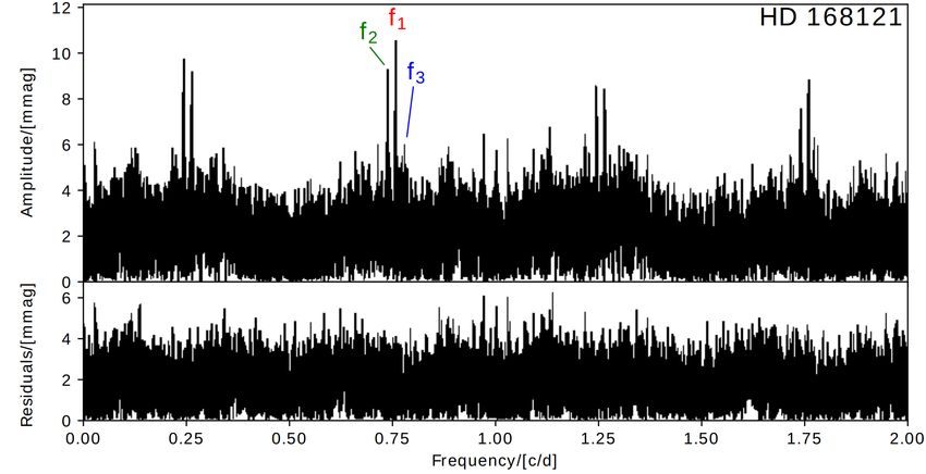
In the case of HD 168121, the spacing between the differ- clearly shows numerous strong emission lines, for instance,
ent overtones n is relatively small for ` = 1 modes. Furthermore, O ii 3728 Å, Hβ 4863 Å, O iii 4960 Å, O iii 5007 Å, Hα 6563 Å,
A122, page 4 of 11M. Fedurco et al.: Pulsational properties of ten new slowly pulsating B stars
Table 2. All detected frequencies along with the corresponding Table 3. Rotation periods for objects with (partially) detected ` = 1
g-modes characterized by angular degree `, radial order ng , and triplets, based on Eq. (1).
azimuthal order m.
Object Period(d)
Frequency Amplitude Phase S /N l ng m
(c/d) (mmag) HD 36999 27.7
HD 66181 21.9(6)
HD 36999 (3.6 M , 25 Myr) HD 97895 16.26(7)
f1 1.50460(2) 10.6(9) 0.41(1) 10.6 1 9 +1
f2 1.43227(2) 12.6(8) 0.66(1) 12.6 1 9 −1
f3 1.82621(3) 5.9(9) 0.84(3) 5.9 1 7 0 and S ii 6716,6731 Å. This is in agreement with the emis-
f4 7.44114(3) 4.6(9) 0.98(3) 4.3 1 1 0 sion profile of the nebula that pervades the corresponding sky
f5 2.61151(3) 4.9(9) 0.17(3) 4.8 1 5 0 region and apparently contaminates the LAMOST spectrum of
HD 48497 (4.2 M , 25 Myr) HD 36999 and the spectra of numerous other stars in the vicinity.
Contamination of LAMOST spectra by H ii regions is a known
f1 0.938(2) 12(4) 0.8(1) 7.0 issue (Hou et al. 2016). We assume that this may be caused by
f2 1.043324(8) 12(2) 0.68(2) 6.6 1 11 fiber drift, issues with the pipeline software responsible for the
f3 0.89578(6) 9(2) 0.01(6) 5.0 1 13 background substraction, or by sampling the background during
f4 1.041(1) 8(3) 0.2(1) 4.5 2 20 the integration while the seeing is excellent.
f5 1.265(1) 8(2) 0.87(5) 4.4 1 9 Because of the higher luminosity derived from Gaia DR2
HD 61076 (3.2 M , 2 Myr) data, we determined that the best-fit model boasts a mass of
f1 1.0919(3) 13(3) 0.4(2) 4.2 1 14 3.6 M and an age of 25 Myr; these values are somewhat higher
f2 2.73251(1) 10(1) 0.35(2) 4.0 1 5 than those given by Wolff et al. (2004) of 3.26 M and 2.2 Myr.
Our analysis suggests a rather low value of fov < 0.01. We
HD 61712 (3.6 M ) achieved best results by regarding frequencies f1 and f2 as
f1 1.281592(3) 18.7(7) 0.422(7) 25.4 1 10 side lobes of a rotationally split triplet. Owing to the non-
f2 1.513(2) 4(1) 0.5(2) 4.7 2 15 detection of the central peak of this supposed triplet and under-
HD 66181 (75 Myr) estimated frequency uncertainties provided by PERIOD04, we
were unable to properly estimate the uncertainty of the rotation
f1 0.88522(2) 14(1) 0.54(1) 11.5 1 12 +1 period.
f2 0.794(8) 9(4) 0.4(2) 7.7 1 12 −1
f3 0.89936(3) 8(1) 0.91(3) 6.6 1 11 0 HD 48497. Niemczura et al. (2009) presented a detailed
f4 0.70470(4) 7(1) 0.52(3) 5.7 2 26 0 abundance analysis of this star, which has a very low υ sin i value
f5 0.84193(3) 6(1) 0.54(3) 4.5 1 12 0 of 13 km s−1 and underabundances of Cr, Sr, and Ni of about
0.5 dex as compared to the solar values. Therefore, Yushchenko
HD 86424 (3.5 M , 50 Myr)
et al. (2015) include HD 48497 in their list of possible λ Bootis
f1 1.084518(3) 12.7(3) 0.544(3) 13.2 1 12 star candidates. These stars constitute a small group of A- to F-
f2 0.10747(1) (a) 4.4(2) 0.873(9) 4.5 type stars characterized by the depletion of Fe-peak elements of
f3 0.95053(4) 4.9(3) 0.50(1) 5.1 1 14 up to 2 dex (Murphy & Paunzen 2017). However, HD 48497 is
HD 97895 (4.8 M , 50 Myr) too hot and does not show the typical elemental abundance pat-
f1 0.922626(7) 16.1(3) 0.667(3) 7.4 1 12 0 tern of λ Bootis stars. It therefore cannot be considered a member
f2 0.861588(8) 15.5(3) 0.471(3) 7.6 1 12 −1 of this group. From our analysis, we find that the models with a
f3 0.98459(1) 10.1(3) 0.275(5) 4.2 1 12 +1 mass of 4.2 M and an age of 25 Myr provide the best fit to the
f4 1.82168(1) 9.3(3) 0.611(5) 4.3 1 6 0
observed frequencies. It is noteworthy that during the analysis,
we discovered that frequency f1 is a side lobe of the 1 d alias
HD 115067 frequency that is ubiquitous in ground-based observations. Con-
f1 0.62165(2) 10(1) 0.15(2) 7.4 1 > 18 sequently, this frequency was disregarded during the grid search
f2 0.18665(2) (a) 7(1) 0.27(2) 4.9 procedure.
HD 163285 (3.8 M , 40 Myr) HD 61076. The available Hipparcos parallax of
f1 0.82863(1) 17.0(8) 0.319(8) 7.1 1 15 0.96(78) mas led to the conclusion that this star is a giant
f2 1.07449(1) 13.3(8) 0.22(1) 5.6 1 11 with a luminosity of 910 L (Hohle et al. 2010). The Gaia
f3 1.20341(1) 11.6(8) 0.94(1) 4.9 2 18 DR2 parallax, on the other hand, places this star well below the
ZAMS. We find that, for the given luminosity, a T eff difference
HD 168121
of 1000 K is needed to shift HD 61076 to the ZAMS for
f1 0.75915(2) 11(1) 0.30(2) 4.9 models with a metallicity of Z = 0.02. The published spectral
f2 0.79316(2) 10(1) 0.99(2) 4.4 type of B5/7 might indicate some peculiarities that render the
f3 0.77929(2) 9(1) 0.06(2) 4.1 temperature estimation uncertain. We strongly suspect that the
T eff determination based on the Gaia DR2 parallax is erroneous;
Notes. Modes were extracted from the best-fit mode combination and
stellar model using a grid of models described in Sect. 4. Masses and however, only further photometric or spectroscopic data can
ages of the stellar models producing the best frequency cross-matches shed more light on this issue and the nature of this star.
are given in parentheses behind the object identifiers. Age estimation Since our grid consists of stellar models with a wide
was carried out in cases where models within 0.5 dex of the best-fit range of metallicity and overshooting parameter values, we
model boasted approximately the same age. (a) Frequency overlap of performed a grid search for the best-fit g-mode combination
synthetic modes too severe to prevent misidentification despite the apparently peculiar nature of this star. As expected,
A122, page 5 of 11A&A 633, A122 (2020)
low-metallicity models with Z < 0.01 were able to shift the be closely matched by dipole modes on 50 Myr old 4.8 M stel-
ZAMS sufficiently toward the position of our object in the HRD. lar models. From the rotational splitting of one of the observed
The best-fit model indicates a 3.2 M object near the ZAMS frequencies, we were able to determine the rotational period.
(2 Myr) with an initially low metallicity of Z = 0.009 and the Despite our expectations, our best-fit models do not indicate
rather high value of fov > 0.03. However, the high value of fov , metallicities significantly different from the solar value. Mod-
the age of the object, and its peculiar location in the HRD cast els with a low value of fov produce a more accurate fit to the
doubt on the reliability of fov . Lack of time on the ZAMS should observed frequencies.
prevent fov from having any significant impact on the internal
structure of the star. In addition, if we exclude models outside HD 115067. With an age of about 90 Myr, this is the most
the 1σ confidence interval, the previously stated constraint on fov evolved star in our sample. Otherwise, no detailed investigations
vanishes (see Fig. C.1). Despite these uncertainties, the scarcity are available in the literature. Unfortunately, in the case of this
of very young SPB stars and the apparently peculiar nature of object, only one frequency suitable for cross-identification was
this object warrant a closer look at HD 61076 in future studies. available, which is insufficient to perform a grid search. Table 2
contains a lower estimate on the radial order of the observed
HD 61712. Mannings & Barlow (1998) presented evidence frequency f1 under the assumption that it corresponds to a dipole
that this star might be a PMS star with significant IR excess. An mode.
inspection of the SED of the object with the VOSA tool clearly
confirms the presence of IR excess. However, a PMS nature can- HD 163285. No detailed investigations of this object are
not be unambiguously established by this criterion alone because available in the literature. High-metallicity stellar models with
similar excesses have been observed in stars that have already a mass of 3.8 M and an age of 40 Myr provide the best fit to the
reached the MS (Montesinos et al. 2009). One definite diag- observed frequencies. The value fov can be constrained within
nostic criterion would be the presence of emission lines; how- the range from 0.024 to 0.030.
ever, to the best of our knowledge, no spectrum of this object HD 168121. No detailed investigations of this object are
is available. Our analysis failed to provide an unambiguous age available in the literature.
estimation because multiple stellar models with similar values
of χ2 were obtained for the best-fit g-mode combination. How-
ever, these models uniformly point to a mass of 3.6 M . In sum- 7. Conclusions
mary, HD 61712 is a candidate young SPB star worthy of further
attention. We collected and analyzed extensive sets of photometric time
series data of ten hitherto unidentified SPB stars with the aim
HD 66181. No detailed investigations of this object are avail- of describing their pulsational properties and identifying pulsa-
able in the literature. Unfortunately, although the best-fit g-mode tional modes. Astrophysical parameters were calculated and the
combination was found, we were unable to put constraints on location of our sample stars in the log T eff vs. log L/L diagram
the mass of the object. However, from the detection of a dipole was investigated. We calculated current pulsational models to
triplet, the rotational period could be calculated (see Table 3). identify pulsational modes in our sample stars. An extensive grid
of stellar models and its corresponding eigenfrequencies were
HD 86424. This star is a visual binary with a magnitude dif-
calculated.
ference of the components (HD 86424 and CD−41 5479B) of
For eight objects, the observed frequencies were successfully
2.3 mag and a separation of 900. 7 (Sinachopoulos 1988). Using the
available Gaia DR2 parallaxes, Bailer-Jones et al. (2018) esti- cross-matched with a best-fit g-mode combination using our grid
mate distances between 547 and 573 pc for HD 86424 and 585 search algorithm. From the best-fit stellar model, we were able
and 607 pc for CD−41 5479B. The two stars, therefore, do not to constrain the astrophysical properties of our sample stars.
form a physical system. Assuming an identical reddening value In the case of five objects (HD 48497, HD 61076, HD 61712,
and the given distance, we derive an absolute magnitude of about HD 86424, and HD 163285), we were able to constrain masses
+2.5 mag for the fainter component. This is typical for a F0 V down to the resolution limit of the grid, i.e., 0.1 M . Employ-
star, which is also compatible with the available optical and near- ing the ages of the corresponding best-fit models (see Table 2),
we were also able to derive information on the age of seven
infrared colors. In this spectral region is situated the blue border
stars. HD 36999 is a particular interesting object because it is
of the γ Doradus instability strip (Bradley et al. 2015), which is
located on, or slightly below, the ZAMS. HD 61712 is another
populated by g-mode pulsators with periods between 0.5 and 5 d.
We are not able to rule out that CD−41 5479B is the source of the candidate young SPB star. A special case is HD 61076, which
detected variability because both stars are covered by the aper- may be a very young and low-metallicity object, according to
tures of the employed data sources. The parameters of the two the best-fit models. On the opposite side, the best-fit models for
best-fit models point to a mass of 2.5 M and an approximate HD 86424 and HD 163285 indicate a higher than average metal-
age of 50 Myr. However, it has to be pointed out that the best-fit licity of 0.027. In accordance with our expectations, no evolved
stellar models within the 1σ confidence interval boast a rather SPB stars are present in our sample.
high metallicity of Z = 0.027. As we do not have any additional As far as overshooting parameter fov is concerned, our results
can be divided into three groups. The first group consists of
information about the metallicity of HD 86424, we are unable to
HD 48497, HD 61712, HD 66181, and HD 86424, and boasts
confirm the validity of our models.
a wide range of best-fit values of fov , which demonstrates the
HD 97895. With a Galactic latitude of +29◦ and low radial need to better constrain this parameter using g-mode pulsations
velocity (Kordopatis et al. 2013), this star is an unusual hot in stars with convective cores. In the second group of objects
B-type star because it is situated most certainly in the thick disk (HD 36999 and HD 97895), there is a clear tendency for mod-
and is characterized by a metallicity significantly different from els with low values of fov to produce better frequency cross-
the solar value (Miranda et al. 2016). The SPB stars of such matches. Finally, in the third group of objects (HD 61076 and
metallicities are valuable testbeds for the calibration of pulsa- HD 163285), the best-fit models confined fov to intervals above
tional models (Miglio et al. 2007). The observed frequencies can 0.02 (see Fig. C.1).
A122, page 6 of 11M. Fedurco et al.: Pulsational properties of ten new slowly pulsating B stars
With the present study, we significantly enlarge the sam- Hou, W., Luo, A.-L., Hu, J.-Y., et al. 2016, Res. Astron. Astrophys., 16,
ple of known SPB stars with reliable pulsational mode identi- 138
fications. We furthermore demonstrate the feasibility of using Houk, N., & Swift, C. 1999, Michigan Spectral Survey, 5
Kharchenko, N. V. 2001, Kinematika i Fizika Nebesnykh Tel, 17, 409
ground-based observations to perform basic asteroseismologi- Kochanek, C. S., Shappee, B. J., Stanek, K. Z., et al. 2017, PASP, 129, 104502
cal analyses of SPB stars. While our results do not reach the Koen, C., & Eyer, L. 2002, MNRAS, 331, 45
accuracy of previous studies based exclusively on space pho- Kordopatis, G., Gilmore, G., Steinmetz, M., et al. 2013, AJ, 146, 134
tometry (e.g., Szewczuk & Daszyńska-Daszkiewicz 2018), they Lenz, P., & Breger, M. 2005, Commun. Asteroseismol., 146, 53
Lindegren, L., Hernández, J., Bombrun, A., et al. 2018, A&A, 616, A2
nevertheless constitute a significant improvement on the con- Mannings, V., & Barlow, M. J. 1998, ApJ, 497, 330
straints provided by the uncertainties in T eff and luminosity Miglio, A., Montalbán, J., & Dupret, M.-A. 2007, MNRAS, 375, L21
derived from photometry and Gaia data. In theory, the presented Miranda, M. S., Pilkington, K., Gibson, B. K., et al. 2016, A&A, 587, A10
approach can also be used with space-based observations. How- Montesinos, B., Eiroa, C., Mora, A., & Merín, B. 2009, A&A, 495, 901
ever, owing to the much higher number of frequencies detected Moravveji, E., Aerts, C., Pápics, P. I., Triana, S. A., & Vandoren, B. 2015, A&A,
580, A27
in these data, the grid search algorithm should be replaced by Moravveji, E., Townsend, R. H. D., Aerts, C., & Mathis, S. 2016, ApJ, 823, 130
a more refined and less computationally heavy cross-matching Murphy, S. J., & Paunzen, E. 2017, MNRAS, 466, 546
algorithm. Such effort may lead to much tighter constraints on Napiwotzki, R., Schoenberner, D., & Wenske, V. 1993, A&A, 268, 653
stellar parameters, which will help to shed more light on the Netopil, M., Paunzen, E., Hümmerich, S., & Bernhard, K. 2017, MNRAS, 468,
2745
internal processes at work in upper MS stars. Nichols, J. S., Henden, A. A., Huenemoerder, D. P., et al. 2010, ApJS, 188, 473
Niemczura, E., Morel, T., & Aerts, C. 2009, A&A, 506, 213
Acknowledgements. The research of M.F. was supported by the Slovak Pápics, P. I., Moravveji, E., Aerts, C., et al. 2014, A&A, 570, A8
Research and Development Agency under the contract No. APVV-15-0458 Pápics, P. I., Tkachenko, A., Aerts, C., et al. 2015, ApJ, 803, L25
and internal grant No. VVGS-PF-2018-758 of the Faculty of Science, P. J. Pápics, P. I., Tkachenko, A., Van Reeth, T., et al. 2017, A&A, 598, A74
Šafárik University in Košice. This work presents results from the European Paunzen, E. 2015, A&A, 580, A23
Space Agency (ESA) space mission Gaia. Gaia data are being processed by Paunzen, E., & Vanmunster, T. 2016, Astron. Nachr., 337, 239
the Gaia Data Processing and Analysis Consortium (DPAC). Funding for the Paxton, B., Bildsten, L., Dotter, A., et al. 2011, ApJS, 192, 3
DPAC is provided by national institutions, in particular the institutions partic- Paxton, B., Cantiello, M., Arras, P., et al. 2013, ApJS, 208, 4
ipating in the Gaia MultiLateral Agreement (MLA). The Gaia mission web- Paxton, B., Marchant, P., Schwab, J., et al. 2015, ApJS, 220, 15
site is https://www.cosmos.esa.int/gaia. The Gaia archive website is Paxton, B., Schwab, J., Bauer, E. B., et al. 2018, ApJS, 234, 34
https://archives.esac.esa.int/gaia. This research has made use of Pecaut, M. J., & Mamajek, E. E. 2013, ApJS, 208, 9
the SIMBAD database and the VizieR catalog access tool, operated at CDS, Pigulski, A. 2014, in Precision Asteroseismology, eds. J. A. Guzik, W. J. Chaplin,
Strasbourg, France. G. Handler, & A. Pigulski, IAU Symp., 301, 31
Preston, G. W. 1974, ARA&A, 12, 257
Ripepi, V., Balona, L., Catanzaro, G., et al. 2015, MNRAS, 454, 2606
References Rivinius, T., Carciofi, A. C., & Martayan, C. 2013, A&ARv, 21, 69
Samus, N. N., Kazarovets, E. V., Durlevich, O. V., Kireeva, N. N., & Pastukhova,
Abt, H. A., Levato, H., & Grosso, M. 2002, ApJ, 573, 359 E. N. 2017, Astron. Rep., 61, 80
Aerts, C., Christensen-Dalsgaard, J., & Kurtz, D. W. 2010, Asteroseismology Sinachopoulos, D. 1988, A&AS, 76, 189
(Netherlands: Springer), 15 Skiff, B. A. 2014, VizieR Online Data Catalog: B/mk
Alfonso-Garzón, J., Domingo, A., & Mas-Hesse, J. M. 2015, in Highlights of Skrutskie, M. F., Cutri, R. M., Stiening, R., et al. 2006, AJ, 131, 1163
Spanish Astrophysics VIII, eds. A. J. Cenarro, F. Figueras, C. Hernández- Street, R. A., Pollaco, D. L., Fitzsimmons, A., et al. 2003, in Scientific Frontiers
Monteagudo, J. Trujillo Bueno, & L. Valdivielso, 435 in Research on Extrasolar Planets, eds. D. Deming, & S. Seager, ASP Conf.
Auvergne, M., Bodin, P., Boisnard, L., et al. 2009, A&A, 506, 411 Ser., 294, 405
Bailer-Jones, C. A. L., Rybizki, J., Fouesneau, M., Mantelet, G., & Andrae, R. Szewczuk, W., & Daszyńska-Daszkiewicz, J. 2018, MNRAS, 478, 2243
2018, AJ, 156, 58 Tian, K. P., van Leeuwen, F., Zhao, J. L., & Su, C. G. 1996, A&AS, 118, 503
Bayo, A., Rodrigo, C., Barrado Y Navascués, D., et al. 2008, A&A, 492, 277 Townsend, R. H. D., & Teitler, S. A. 2013, MNRAS, 435, 3406
Borucki, W. J. 2016, Rep. Progr. Phys., 79, 036901 Townsend, R. H. D., Goldstein, J., & Zweibel, E. G. 2018, MNRAS, 475, 879
Bradley, P. A., Guzik, J. A., Miles, L. F., et al. 2015, AJ, 149, 68 Triana, S. A., Moravveji, E., Pápics, P. I., et al. 2015, ApJ, 810, 16
Buysschaert, B., Aerts, C., Bowman, D. M., et al. 2018, A&A, 616, A148 van Leeuwen, F. 1997, in Hipparcos – Venice ’97, eds. R. M. Bonnet, E. Høg,
Castro, N., Fossati, L., Langer, N., et al. 2014, A&A, 570, L13 P. L. Bernacca, et al., ESA SP, 402, 19
Cowling, T. G., & Newing, R. A. 1949, ApJ, 109, 149 Waelkens, C. 1991, A&A, 246, 453
Cui, X.-Q., Zhao, Y.-H., Chu, Y.-Q., et al. 2012, Res. Astron. Astrophys., 12, Watson, C. L., Henden, A. A., & Price, A. 2006, Soc. Astron. Sci. Ann. Symp.,
1197 25, 47
De Cat, P. 2007, Commun. Asteroseismol., 150, 167 Wenger, M., Ochsenbein, F., Egret, D., et al. 2000, A&AS, 143, 9
Degroote, P., Acke, B., Samadi, R., et al. 2011, A&A, 536, A82 Wolff, S. C., Strom, S. E., & Hillenbrand, L. A. 2004, ApJ, 601, 979
Dolginov, A. Z., & Urpin, V. A. 1983, Ap&SS, 95, 1 Yushchenko, A. V., Gopka, V. F., Kang, Y.-W., et al. 2015, AJ, 149, 59
ESA 1997, in The HIPPARCOS and TYCHO Catalogues. Astrometric and Zhao, G., Zhao, Y.-H., Chu, Y.-Q., Jing, Y.-P., & Deng, L.-C. 2012, Res. Astron.
Photometric Star Catalogues Derived from the ESA Hipparcos Space Astrophys., 12, 723
Astrometry Mission, ESA SP, 1200 Zwintz, K., Hareter, M., Kuschnig, R., et al. 2009, A&A, 502, 239
Flower, P. J. 1996, ApJ, 469, 355 Zwintz, K., Fossati, L., Ryabchikova, T., et al. 2013, A&A, 550, A121
Gautschy, A., & Saio, H. 1993, MNRAS, 262, 213 Zwintz, K., Fossati, L., & Ryabchikova, T. 2015, in Physics and Evolution of
Green, G. M., Schlafly, E. F., Finkbeiner, D., et al. 2018, MNRAS, 478, 651 Magnetic and Related Stars, eds. Y. Y. Balega, I. I. Romanyuk, & D. O.
Gruber, D., Saio, H., Kuschnig, R., et al. 2012, MNRAS, 420, 291 Kudryavtsev, ASP Conf. Ser., 494, 157
Hohle, M. M., Neuhäuser, R., & Schutz, B. F. 2010, Astron. Nachr., 331, 349 Zwintz, K., Moravveji, E., Pápics, P. I., et al. 2017, A&A, 601, A101
A122, page 7 of 11A&A 633, A122 (2020)
Appendix A: Amplitude spectra
14 f2 f1 HD 36999 14
f1 f2 HD 48497
12
f4
12
Am plit ude/[ m m ag]
Am plit ude/[ m m ag]
f3 f5
10 10
f3 f4 8
8
f5
6 6
4 4
2 2
Residuals/[ m m ag]
Residuals/[ m m ag]
0 6
4
4
2
2
0 0
0 1 2 3 4 5 6 7 8 0.00 0.25 0.50 0.75 1.00 1.25 1.50 1.75 2.00
15.0 f1 HD 61076 20 f1 HD 61712
2fNyq - (f1 +5)
Am plit ude/[ m m ag]
Am plit ude/[ m m ag]
12.5
f2 15
10.0
2fNyq - (f1 +4)
2fNyq - (f1 +3)
7.5 10
5.0
f2
5
2.5
Residuals/[ m m ag]
Residuals/[ m m ag]
0.0 0
7.5 3
5.0 2
2.5 1
0.0 0
0.0 0.5 1.0 1.5 2.0 2.5 3.0 0.0 0.5 1.0 1.5 2.0 2.5 3.0
14
f1 HD 66181 f1 HD 86424
14
12
Am plit ude/[ m m ag]
Am plit ude/[ m m ag]
12
10
10 f2 f3 f3
f4 8
f2
8
f5 6
6
4
4
2 2
Residuals/[ m m ag]
Residuals/[ m m ag]
0 3
4
2
2
1
0 0
0.00 0.25 0.50 0.75 1.00 1.25 1.50 1.75 2.00 0.0 0.5 1.0 1.5 2.0 2.5 3.0
17.5
f 2f 1 HD 97895 f1 HD 115067
10
15.0
f4
Am plit ude/[ m m ag]
Am plit ude/[ m m ag]
12.5 f3 8
f2
10.0
6
7.5
4
5.0
2
2.5
Residuals/[ m m ag]
Residuals/[ m m ag]
6 0
6
4 4
2 2
0 0
0.0 0.5 1.0 1.5 2.0 2.5 3.0 0.0 0.2 0.4 0.6 0.8 1.0
f1 HD 163285
17.5
15.0 f2
Am plit ude/[ m m ag]
12.5 f3
10.0
7.5
5.0
2.5
0.0
Residuals/[ m m ag]
4
2
0
0.00 0.25 0.50 0.75 1.00 1.25 1.50 1.75 2.00
Frequency/[ c/d]
Fig. A.1. Results of the frequency analysis of the light curves of our sample stars. The top panels of each plot illustrate the original amplitude
spectra. Significant frequencies, as listed in Table 2, are identified. The bottom panels shows the residuals after subtracting the indicated frequencies
and corresponding aliases.
A122, page 8 of 11M. Fedurco et al.: Pulsational properties of ten new slowly pulsating B stars
Appendix B: MESA and Gyre inlists tol_max_correction = 1d-7
/ ! end of controls namelist
The grid of stellar models was produced using the following
MESA inlist file. Empty parameter values were filled sequen- After the grid of stellar models was created, each stellar
tially for each node of the grid. model was then used to calculate the frequencies of dipole and
quadrupole g-modes using the following GYRE inlist:
&star_job
create_pre_main_sequence_model = .false. /
write_profile_when_terminate = .false. &model
show_log_description_at_start = .false. model_type = ’EVOL’
change_lnPgas_flag = .true. file =
change_initial_lnPgas_flag = .true. file_format = ’MESA’
new_lnPgas_flag = .true. uniform_rot = .TRUE.
change_Z = .true. Omega_units = ’CYC_PER_DAY’
change_initial_Z = .true. Omega_rot = 0.0
new_z = repair_As = .TRUE.
/ !end of star_job namelist /
&constants
&controls /
write_profiles_flag = .true. &mode
profile_interval = 15 l = 1
history_interval = 3 n_pg_min = -25
write_header_frequency = 999999 tag = ’l=1’
terminal_interval = 999999 /
photo_interval = 5000000 &mode
log_directory = l = 2
n_pg_min = -30
initial_mass = tag = ’l=2’
mixing_length_alpha = 1.73 /
set_min_D_mix = .true. &osc
min_D_mix = 0 nonadiabatic = .TRUE.
/
overshoot_f_above_burn_h_core = &num
overshoot_f0_above_burn_h_core = 0.005 diff_scheme = ’COLLOC_GL4’
dX_div_X_hard_limit = 1d-3 /
&scan
delta_lg_XH_cntr_max = -1 grid_type = ’INVERSE’
delta_lg_XH_cntr_limit = 0.05 freq_min_units = ’CYC_PER_DAY’
freq_max_units = ’CYC_PER_DAY’
alpha_semiconvection = 0.01 freq_min = 0.321
write_pulse_data_with_profile = .true. freq_max = 10.0
pulse_data_format = "GYRE" n_freq = 100
add_center_point_to_pulse_data = .true. tag_list = ’l=1’
add_double_points_to_pulse_data = .true. /
calculate_Brunt_N2 = .true. &scan
xa_central_lower_limit_species(1) = "h1" grid_type = ’INVERSE’
xa_central_lower_limit(1) = 1d-3 freq_min_units = ’CYC_PER_DAY’
freq_max_units = ’CYC_PER_DAY’
when_to_stop_rtol = 1d-3 freq_min = 0.6
when_to_stop_atol = 1d-3 freq_max = 10.0
n_freq = 100
mixing_D_limit_for_log = 1d-4 tag_list = ’l=2’
use_Ledoux_criterion = .true. /
D_mix_ov_limit = 0d0 &grid
which_atm_option = "photosphere_tables" alpha_osc = 10
cubic_interpolation_in_Z = .true. alpha_exp = 2
n_inner = 5
! test with "Gold Standard" tolerances /
threshold_grad_mu_for_double_point = 10. &nad_output
newton_iterations_limit = 20 summary_file =
max_tries = 20 freq_units = ’CYC_PER_DAY’
iter_for_resid_tol2 = 30 summary_file_format = ’TXT’
tol_residual_norm1 = 1d-9 summary_item_list = ’M_star,R_star,l,m,n_pg,
tol_max_residual1 = 1d-7 n_p,n_g,freq,freq_units,E,E_norm,eta’
tol_correction_norm = 1d-9 /
A122, page 9 of 11A&A 633, A122 (2020)
Appendix C: χ2 distributions for the best-fit g-mode combinations
HD 36999 HD 48497
HD 61076 HD 61712
HD 66181 HD 86424
Fig. C.1. χ2 values of stellar models within 1σ (blue points) and 3σ (gray points) of the given target. Represented χ2 values were calculated for
the best-fit g-mode combination as listed in Table 2. Each figure shows the χ2 distribution across all free parameters of the stellar model grid, i.e.,
initial mass (top left), age (top right), metallicity (bottom left), and overshooting (bottom right).
A122, page 10 of 11M. Fedurco et al.: Pulsational properties of ten new slowly pulsating B stars
HD 97895 HD 163285
Fig. C.1. continued.
A122, page 11 of 11You can also read