Learning Transferable Architectures for Scalable Image Recognition
←
→
Page content transcription
If your browser does not render page correctly, please read the page content below
Learning Transferable Architectures for Scalable Image Recognition

                                                      Barret Zoph                   Vijay Vasudevan               Jonathon Shlens                  Quoc V. Le
                                                      Google Brain                   Google Brain                  Google Brain                   Google Brain
                                               barretzoph@google.com                vrv@google.com               shlens@google.com              qvl@google.com
arXiv:1707.07012v4 [cs.CV] 11 Apr 2018

                                                                 Abstract                                    1. Introduction
                                                                                                                 Developing neural network image classification models
                                                                                                             often requires significant architecture engineering. Starting
                                             Developing neural network image classification models           from the seminal work of [32] on using convolutional archi-
                                         often requires significant architecture engineering. In this        tectures [17, 34] for ImageNet [11] classification, succes-
                                         paper, we study a method to learn the model architectures           sive advancements through architecture engineering have
                                         directly on the dataset of interest. As this approach is ex-        achieved impressive results [53, 59, 20, 60, 58, 68].
                                         pensive when the dataset is large, we propose to search for             In this paper, we study a new paradigm of designing con-
                                         an architectural building block on a small dataset and then         volutional architectures and describe a scalable method to
                                         transfer the block to a larger dataset. The key contribu-           optimize convolutional architectures on a dataset of inter-
                                         tion of this work is the design of a new search space (which        est, for instance the ImageNet classification dataset. Our
                                         we call the “NASNet search space”) which enables trans-             approach is inspired by the recently proposed Neural Ar-
                                         ferability. In our experiments, we search for the best con-         chitecture Search (NAS) framework [71], which uses a re-
                                         volutional layer (or “cell”) on the CIFAR-10 dataset and            inforcement learning search method to optimize architec-
                                         then apply this cell to the ImageNet dataset by stacking to-        ture configurations. Applying NAS, or any other search
                                         gether more copies of this cell, each with their own parame-        methods, directly to a large dataset, such as the ImageNet
                                         ters to design a convolutional architecture, which we name          dataset, is however computationally expensive. We there-
                                         a “NASNet architecture”. We also introduce a new regu-              fore propose to search for a good architecture on a proxy
                                         larization technique called ScheduledDropPath that signif-          dataset, for example the smaller CIFAR-10 dataset, and then
                                         icantly improves generalization in the NASNet models. On            transfer the learned architecture to ImageNet. We achieve
                                         CIFAR-10 itself, a NASNet found by our method achieves              this transferrability by designing a search space (which we
                                         2.4% error rate, which is state-of-the-art. Although the cell       call “the NASNet search space”) so that the complexity of
                                         is not searched for directly on ImageNet, a NASNet con-             the architecture is independent of the depth of the network
                                         structed from the best cell achieves, among the published           and the size of input images. More concretely, all convolu-
                                         works, state-of-the-art accuracy of 82.7% top-1 and 96.2%           tional networks in our search space are composed of convo-
                                         top-5 on ImageNet. Our model is 1.2% better in top-1 accu-          lutional layers (or “cells”) with identical structure but dif-
                                         racy than the best human-invented architectures while hav-          ferent weights. Searching for the best convolutional archi-
                                         ing 9 billion fewer FLOPS – a reduction of 28% in compu-            tectures is therefore reduced to searching for the best cell
                                         tational demand from the previous state-of-the-art model.           structure. Searching for the best cell structure has two main
                                         When evaluated at different levels of computational cost,           benefits: it is much faster than searching for an entire net-
                                         accuracies of NASNets exceed those of the state-of-the-art          work architecture and the cell itself is more likely to gener-
                                         human-designed models. For instance, a small version of             alize to other problems. In our experiments, this approach
                                         NASNet also achieves 74% top-1 accuracy, which is 3.1%              significantly accelerates the search for the best architectures
                                         better than equivalently-sized, state-of-the-art models for         using CIFAR-10 by a factor of 7× and learns architectures
                                         mobile platforms. Finally, the image features learned from          that successfully transfer to ImageNet.
                                         image classification are generically useful and can be trans-           Our main result is that the best architecture found on
                                         ferred to other computer vision problems. On the task of ob-        CIFAR-10, called NASNet, achieves state-of-the-art ac-
                                         ject detection, the learned features by NASNet used with the        curacy when transferred to ImageNet classification with-
                                         Faster-RCNN framework surpass state-of-the-art by 4.0%              out much modification. On ImageNet, NASNet achieves,
                                         achieving 43.1% mAP on the COCO dataset.                            among the published works, state-of-the-art accuracy of
                                                                                                             82.7% top-1 and 96.2% top-5. This result amounts to a

                                                                                                         1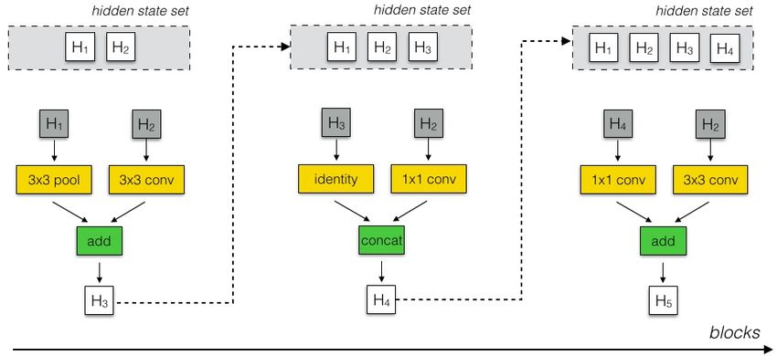
1.2% improvement in top-1 accuracy than the best human-         3. Method
invented architectures while having 9 billion fewer FLOPS.
On CIFAR-10 itself, NASNet achieves 2.4% error rate,               Our work makes use of search methods to find good con-
which is also state-of-the-art.                                 volutional architectures on a dataset of interest. The main
                                                                search method we use in this work is the Neural Architec-
   Additionally, by simply varying the number of the con-       ture Search (NAS) framework proposed by [71]. In NAS,
volutional cells and number of filters in the convolutional     a controller recurrent neural network (RNN) samples child
cells, we can create different versions of NASNets with dif-    networks with different architectures. The child networks
ferent computational demands. Thanks to this property of        are trained to convergence to obtain some accuracy on a
the cells, we can generate a family of models that achieve      held-out validation set. The resulting accuracies are used
accuracies superior to all human-invented models at equiv-      to update the controller so that the controller will generate
alent or smaller computational budgets [60, 29]. Notably,       better architectures over time. The controller weights are
the smallest version of NASNet achieves 74.0% top-1 ac-         updated with policy gradient (see Figure 1).
curacy on ImageNet, which is 3.1% better than previously
engineered architectures targeted towards mobile and em-                                   Sample architecture A!
bedded vision tasks [24, 70].                                                                with probability p

   Finally, we show that the image features learned by
NASNets are generically useful and transfer to other com-                                                              Train a child network!
                                                                                                                       with architecture A to !
puter vision problems. In our experiments, the features             The controller (RNN)
                                                                                                                        convergence to get !
learned by NASNets from ImageNet classification can be                                                                 validation accuracy R
combined with the Faster-RCNN framework [47] to achieve
state-of-the-art on COCO object detection task for both the
                                                                                           Scale gradient of p by R!
largest as well as mobile-optimized models. Our largest                                    to update the controller

NASNet model achieves 43.1% mAP, which is 4% better
than previous state-of-the-art.                                 Figure 1. Overview of Neural Architecture Search [71]. A con-
                                                                troller RNN predicts architecture A from a search space with prob-
                                                                ability p. A child network with architecture A is trained to con-
                                                                vergence achieving accuracy R. Scale the gradients of p by R to
2. Related Work
                                                                update the RNN controller.
    The proposed method is related to previous work in hy-
perparameter optimization [44, 4, 5, 54, 55, 6, 40] – es-
                                                                    The main contribution of this work is the design of a
pecially recent approaches in designing architectures such
                                                                novel search space, such that the best architecture found
as Neural Fabrics [48], DiffRNN [41], MetaQNN [3] and
                                                                on the CIFAR-10 dataset would scale to larger, higher-
DeepArchitect [43]. A more flexible class of methods for
                                                                resolution image datasets across a range of computational
designing architecture is evolutionary algorithms [65, 16,
                                                                settings. We name this search space the NASNet search
57, 30, 46, 42, 67], yet they have not had as much success
                                                                space as it gives rise to NASNet, the best architecture found
at large scale. Xie and Yuille [67] also transferred learned
                                                                in our experiments. One inspiration for the NASNet search
architectures from CIFAR-10 to ImageNet but performance
                                                                space is the realization that architecture engineering with
of these models (top-1 accuracy 72.1%) are notably below
                                                                CNNs often identifies repeated motifs consisting of com-
previous state-of-the-art (Table 2).
                                                                binations of convolutional filter banks, nonlinearities and a
   The concept of having one neural network interact with a     prudent selection of connections to achieve state-of-the-art
second neural network to aid the learning process, or learn-    results (such as the repeated modules present in the Incep-
ing to learn or meta-learning [23, 49] has attracted much       tion and ResNet models [59, 20, 60, 58]). These observa-
attention in recent years [1, 62, 14, 19, 35, 45, 15]. Most     tions suggest that it may be possible for the controller RNN
of these approaches have not been scaled to large problems      to predict a generic convolutional cell expressed in terms of
like ImageNet. An exception is the recent work focused          these motifs. This cell can then be stacked in series to han-
on learning an optimizer for ImageNet classification that       dle inputs of arbitrary spatial dimensions and filter depth.
achieved notable improvements [64].                                 In our approach, the overall architectures of the convo-
   The design of our search space took much inspira-            lutional nets are manually predetermined. They are com-
tion from LSTMs [22], and Neural Architecture Search            posed of convolutional cells repeated many times where
Cell [71]. The modular structure of the convolutional cell is   each convolutional cell has the same architecture, but dif-
also related to previous methods on ImageNet such as VGG        ferent weights. To easily build scalable architectures for
[53], Inception [59, 60, 58], ResNet/ResNext [20, 68], and      images of any size, we need two types of convolutional cells
Xception/MobileNet [9, 24].                                     to serve two main functions when taking in a feature map
the Normal and Reduction Cells, which are searched by the
controller RNN. The structures of the cells can be searched
within a search space defined as follows (see Appendix,
Figure 7 for schematic). In our search space, each cell re-
ceives as input two initial hidden states hi and hi−1 which
are the outputs of two cells in previous two lower layers
or the input image. The controller RNN recursively pre-
dicts the rest of the structure of the convolutional cell, given
these two initial hidden states (Figure 3). The predictions
of the controller for each cell are grouped into B blocks,
where each block has 5 prediction steps made by 5 distinct
softmax classifiers corresponding to discrete choices of the
elements of a block:
Step 1. Select a hidden state from hi , hi−1 or from the set of hidden
states created in previous blocks.
Step 2. Select a second hidden state from the same options as in Step 1.
Step 3. Select an operation to apply to the hidden state selected in Step 1.
Step 4. Select an operation to apply to the hidden state selected in Step 2.
Figure 2. Scalable architectures for image classification consist of Step 5. Select a method to combine the outputs of Step 3 and 4 to create
two repeated motifs termed Normal Cell and Reduction Cell. This a new hidden state.
diagram highlights the model architecture for CIFAR-10 and Ima-
geNet. The choice for the number of times the Normal Cells that The algorithm appends the newly-created hidden state to
gets stacked between reduction cells, N , can vary in our experi- the set of existing hidden states as a potential input in sub-
ments. sequent blocks. The controller RNN repeats the above 5
prediction steps B times corresponding to the B blocks in
a convolutional cell. In our experiments, selecting B = 5
provides good results, although we have not exhaustively
as input: (1) convolutional cells that return a feature map of
searched this space due to computational limitations.
the same dimension, and (2) convolutional cells that return
In steps 3 and 4, the controller RNN selects an operation
a feature map where the feature map height and width is re-
to apply to the hidden states. We collected the following set
duced by a factor of two. We name the first type and second
of operations based on their prevalence in the CNN litera-
type of convolutional cells Normal Cell and Reduction Cell
ture:
respectively. For the Reduction Cell, we make the initial
operation applied to the cell’s inputs have a stride of two to • identity • 1x3 then 3x1 convolution
reduce the height and width. All of our operations that we • 1x7 then 7x1 convolution • 3x3 dilated convolution
consider for building our convolutional cells have an option • 3x3 average pooling • 3x3 max pooling
• 5x5 max pooling • 7x7 max pooling
of striding. • 1x1 convolution • 3x3 convolution
Figure 2 shows our placement of Normal and Reduction • 3x3 depthwise-separable conv • 5x5 depthwise-seperable conv
Cells for CIFAR-10 and ImageNet. Note on ImageNet we • 7x7 depthwise-separable conv
have more Reduction Cells, since the incoming image size
is 299x299 compared to 32x32 for CIFAR. The Reduction In step 5 the controller RNN selects a method to combine
and Normal Cell could have the same architecture, but we the two hidden states, either (1) element-wise addition be-
empirically found it beneficial to learn two separate archi- tween two hidden states or (2) concatenation between two
tectures. We use a common heuristic to double the number hidden states along the filter dimension. Finally, all of the
of filters in the output whenever the spatial activation size is unused hidden states generated in the convolutional cell are
reduced in order to maintain roughly constant hidden state concatenated together in depth to provide the final cell out-
dimension [32, 53]. Importantly, much like Inception and put.
ResNet models [59, 20, 60, 58], we consider the number of To allow the controller RNN to predict both Normal Cell
motif repetitions N and the number of initial convolutional and Reduction Cell, we simply make the controller have
filters as free parameters that we tailor to the scale of an 2 × 5B predictions in total, where the first 5B predictions
image classification problem. are for the Normal Cell and the second 5B predictions are
What varies in the convolutional nets is the structures of for the Reduction Cell.softmax!
new hidden layer
layer
Select one! Select second! Select operation for ! Select operation for! Select method to!
hidden state hidden state first hidden state second hidden state combine hidden state
hidden layer
add
controller!
3 x 3 conv 2 x 2 maxpool
hidden layer A hidden layer B
repeat B times
Figure 3. Controller model architecture for recursively constructing one block of a convolutional cell. Each block requires selecting 5
discrete parameters, each of which corresponds to the output of a softmax layer. Example constructed block shown on right. A convolu-
tional cell contains B blocks, hence the controller contains 5B softmax layers for predicting the architecture of a convolutional cell. In our
experiments, the number of blocks B is 5.
Finally, our work makes use of the reinforcement learn- convolutions and the number of branches compared with
ing proposal in NAS [71]; however, it is also possible to competing architectures [53, 59, 20, 60, 58]. Subsequent
use random search to search for architectures in the NAS- experiments focus on this convolutional cell architecture,
Net search space. In random search, instead of sampling although we examine the efficacy of other, top-ranked con-
the decisions from the softmax classifiers in the controller volutional cells in ImageNet experiments (described in Ap-
RNN, we can sample the decisions from the uniform distri- pendix B) and report their results as well. We call the three
bution. In our experiments, we find that random search is networks constructed from the best three searches NASNet-
slightly worse than reinforcement learning on the CIFAR- A, NASNet-B and NASNet-C.
10 dataset. Although there is value in using reinforcement
learning, the gap is smaller than what is found in the original
work of [71]. This result suggests that 1) the NASNet search We demonstrate the utility of the convolutional cells by
space is well-constructed such that random search can per- employing this learned architecture on CIFAR-10 and a
form reasonably well and 2) random search is a difficult family of ImageNet classification tasks. The latter family of
baseline to beat. We will compare reinforcement learning tasks is explored across a few orders of magnitude in com-
against random search in Section 4.4. putational budget. After having learned the convolutional
cells, several hyper-parameters may be explored to build a
final network for a given task: (1) the number of cell repeats
4. Experiments and Results
N and (2) the number of filters in the initial convolutional
In this section, we describe our experiments with the cell. After selecting the number of initial filters, we use a
method described above to learn convolutional cells. In common heuristic to double the number of filters whenever
summary, all architecture searches are performed using the the stride is 2. Finally, we define a simple notation, e.g.,
CIFAR-10 classification task [31]. The controller RNN was 4 @ 64, to indicate these two parameters in all networks,
trained using Proximal Policy Optimization (PPO) [51] by where 4 and 64 indicate the number of cell repeats and the
employing a global workqueue system for generating a pool number of filters in the penultimate layer of the network,
of child networks controlled by the RNN. In our experi- respectively.
ments, the pool of workers in the workqueue consisted of
500 GPUs.
For complete details of of the architecture learning algo-
The result of this search process over 4 days yields sev-
rithm and the controller system, please refer to Appendix A.
eral candidate convolutional cells. We note that this search
Importantly, when training NASNets, we discovered Sched-
procedure is almost 7× faster than previous approaches [71]
uledDropPath, a modified version of DropPath [33], to be
that took 28 days.1 Additionally, we demonstrate below that
an effective regularization method for NASNet. In Drop-
the resulting architecture is superior in accuracy.
Path [33], each path in the cell is stochastically dropped
Figure 4 shows a diagram of the top performing Normal
with some fixed probability during training. In our mod-
Cell and Reduction Cell. Note the prevalence of separable
ified version, ScheduledDropPath, each path in the cell is
1 In particular, we note that previous architecture search [71] used 800 dropped out with a probability that is linearly increased
GPUs for 28 days resulting in 22,400 GPU-hours. The method in this pa- over the course of training. We find that DropPath does not
per uses 500 GPUs across 4 days resulting in 2,000 GPU-hours. The for-
mer effort used Nvidia K40 GPUs, whereas the current efforts used faster
work well for NASNets, while ScheduledDropPath signifi-
NVidia P100s. Discounting the fact that the we use faster hardware, we cantly improves the final performance of NASNets in both
estimate that the current procedure is roughly about 7× more efficient. CIFAR and ImageNet experiments.hi+1
concat
hi+1
add add
concat
max! sep! avg! iden!
3x3 3x3 3x3 tity
add add add add add
add add add
sep! iden! sep! sep! avg! iden! avg! avg! sep! sep! sep! sep! max! sep! avg! sep!
3x3 tity 3x3 5x5 3x3 tity 3x3 3x3 5x5 3x3 7x7 5x5 3x3 7x7 3x3 5x5
hi hi
... ...
hi-1 hi-1
Normal Cell Reduction Cell
Figure 4. Architecture of the best convolutional cells (NASNet-A) with B = 5 blocks identified with CIFAR-10 . The input (white) is the
hidden state from previous activations (or input image). The output (pink) is the result of a concatenation operation across all resulting
branches. Each convolutional cell is the result of B blocks. A single block is corresponds to two primitive operations (yellow) and a
combination operation (green). Note that colors correspond to operations in Figure 3.
4.1. Results on CIFAR-10 Image Classification CNNs hand-designed for this operating regime [24, 70].
Note we do not have residual connections between con-
For the task of image classification with CIFAR-10, we
volutional cells as the models learn skip connections on
set N = 4 or 6 (Figure 2). The test accuracies of the
their own. We empirically found manually inserting resid-
best architectures are reported in Table 1 along with other
ual connections between cells to not help performance. Our
state-of-the-art models. As can be seen from the Table, a
training setup on ImageNet is similar to [60], but please see
large NASNet-A model with cutout data augmentation [12]
Appendix A for details.
achieves a state-of-the-art error rate of 2.40% (averaged
Table 2 shows that the convolutional cells discov-
across 5 runs), which is slightly better than the previous
ered with CIFAR-10 generalize well to ImageNet prob-
best record of 2.56% by [12]. The best single run from our
lems. In particular, each model based on the convolu-
model achieves 2.19% error rate.
tional cells exceeds the predictive performance of the cor-
4.2. Results on ImageNet Image Classification responding hand-designed model. Importantly, the largest
model achieves a new state-of-the-art performance for Ima-
We performed several sets of experiments on ImageNet geNet (82.7%) based on single, non-ensembled predictions,
with the best convolutional cells learned from CIFAR-10. surpassing previous best published result by ∼1.2% [8].
We emphasize that we merely transfer the architectures Among the unpublished works, our model is on par with
from CIFAR-10 but train all ImageNet models weights from the best reported result of 82.7% [25], while having signif-
scratch. icantly fewer floating point operations. Figure 5 shows a
Results are summarized in Table 2 and 3 and Figure 5. complete summary of our results in comparison with other
In the first set of experiments, we train several image clas- published results. Note the family of models based on con-
sification systems operating on 299x299 or 331x331 reso- volutional cells provides an envelope over a broad class of
lution images with different experiments scaled in compu- human-invented architectures.
tational demand to create models that are roughly on par Finally, we test how well the best convolutional cells
in computational cost with Inception-v2 [29], Inception-v3 may perform in a resource-constrained setting, e.g., mobile
[60] and PolyNet [69]. We show that this family of mod- devices (Table 3). In these settings, the number of float-
els achieve state-of-the-art performance with fewer floating ing point operations is severely constrained and predictive
point operations and parameters than comparable architec- performance must be weighed against latency requirements
tures. Second, we demonstrate that by adjusting the scale on a device with limited computational resources. Mo-
of the model we can achieve state-of-the-art performance bileNet [24] and ShuffleNet [70] provide state-of-the-art re-
at smaller computational budgets, exceeding streamlined sults obtaining 70.6% and 70.9% accuracy, respectively onmodel depth # params error rate (%)
DenseNet (L = 40, k = 12) [26] 40 1.0M 5.24
DenseNet(L = 100, k = 12) [26] 100 7.0M 4.10
DenseNet (L = 100, k = 24) [26] 100 27.2M 3.74
DenseNet-BC (L = 100, k = 40) [26] 190 25.6M 3.46
Shake-Shake 26 2x32d [18] 26 2.9M 3.55
Shake-Shake 26 2x96d [18] 26 26.2M 2.86
Shake-Shake 26 2x96d + cutout [12] 26 26.2M 2.56
NAS v3 [71] 39 7.1M 4.47
NAS v3 [71] 39 37.4M 3.65
NASNet-A (6 @ 768) - 3.3M 3.41
NASNet-A (6 @ 768) + cutout - 3.3M 2.65
NASNet-A (7 @ 2304) - 27.6M 2.97
NASNet-A (7 @ 2304) + cutout - 27.6M 2.40
NASNet-B (4 @ 1152) - 2.6M 3.73
NASNet-C (4 @ 640) - 3.1M 3.59
Table 1. Performance of Neural Architecture Search and other state-of-the-art models on CIFAR-10. All results for NASNet are the mean
accuracy across 5 runs.
85 85
NASNet-A (6 @ 4032) NASNet-A (6 @ 4032)
DPN-131
NASNet-A (7 @ 1920) SENet NASNet-A (7 @ 1920) SENet
DPN-131 Inception-ResNet-v2 PolyNet
PolyNet
accuracy (precision @1)
ResNeXt-101 80
accuracy (precision @1)
80 NASNet-A (5 @ 1538) Inception-ResNet-v2 NASNet-A (5 @ 1538) Inception-v4 ResNeXt-101
Inception-v4 Xception
Xception ResNet-152 Inception-v3
Inception-v3
ResNet-152
75 Inception-v2
75 Inception-v2
NASNet-A (4 @ 1056) NASNet-A (4 @ 1056)
VGG-16 VGG-16
ShuffleNet ShuffleNet
MobileNet MobileNet
70 Inception-v1 70 Inception-v1
65 65
0 10000 20000 30000 40000 0 20 40 60 80 100 120 140
# Mult-Add operations (millions) # parameters (millions)
Figure 5. Accuracy versus computational demand (left) and number of parameters (right) across top performing published CNN architec-
tures on ImageNet 2012 ILSVRC challenge prediction task. Computational demand is measured in the number of floating-point multiply-
add operations to process a single image. Black circles indicate previously published results and red squares highlight our proposed
models.
224x224 images using ∼550M multliply-add operations. lems [13]. One of the most important problems is the spa-
An architecture constructed from the best convolutional tial localization of objects within an image. To further
cells achieves superior predictive performance (74.0% ac- validate the performance of the family of NASNet-A net-
curacy) surpassing previous models but with comparable works, we test whether object detection systems derived
computational demand. In summary, we find that the from NASNet-A lead to improvements in object detection
learned convolutional cells are flexible across model scales [28].
achieving state-of-the-art performance across almost 2 or-
ders of magnitude in computational budget. To address this question, we plug in the family of
NASNet-A networks pretrained on ImageNet into the
4.3. Improved features for object detection Faster-RCNN object detection pipeline [47] using an open-
source software platform [28]. We retrain the resulting ob-
Image classification networks provide generic image fea- ject detection pipeline on the combined COCO training plus
tures that may be transferred to other computer vision prob- validation dataset excluding 8,000 mini-validation images.Model image size # parameters Mult-Adds Top 1 Acc. (%) Top 5 Acc. (%)
Inception V2 [29] 224×224 11.2 M 1.94 B 74.8 92.2
NASNet-A (5 @ 1538) 299×299 10.9 M 2.35 B 78.6 94.2
Inception V3 [60] 299×299 23.8 M 5.72 B 78.8 94.4
Xception [9] 299×299 22.8 M 8.38 B 79.0 94.5
Inception ResNet V2 [58] 299×299 55.8 M 13.2 B 80.1 95.1
NASNet-A (7 @ 1920) 299×299 22.6 M 4.93 B 80.8 95.3
ResNeXt-101 (64 x 4d) [68] 320×320 83.6 M 31.5 B 80.9 95.6
PolyNet [69] 331×331 92 M 34.7 B 81.3 95.8
DPN-131 [8] 320×320 79.5 M 32.0 B 81.5 95.8
SENet [25] 320×320 145.8 M 42.3 B 82.7 96.2
NASNet-A (6 @ 4032) 331×331 88.9 M 23.8 B 82.7 96.2
Table 2. Performance of architecture search and other published state-of-the-art models on ImageNet classification. Mult-Adds indicate
the number of composite multiply-accumulate operations for a single image. Note that the composite multiple-accumulate operations are
calculated for the image size reported in the table. Model size for [25] calculated from open-source implementation.
Model # parameters Mult-Adds Top 1 Acc. (%) Top 5 Acc. (%)
†
Inception V1 [59] 6.6M 1,448 M 69.8 89.9
MobileNet-224 [24] 4.2 M 569 M 70.6 89.5
ShuffleNet (2x) [70] ∼ 5M 524 M 70.9 89.8
NASNet-A (4 @ 1056) 5.3 M 564 M 74.0 91.6
NASNet-B (4 @ 1536) 5.3M 488 M 72.8 91.3
NASNet-C (3 @ 960) 4.9M 558 M 72.5 91.0
Table 3. Performance on ImageNet classification on a subset of models operating in a constrained computational setting, i.e., < 1.5 B
multiply-accumulate operations per image. All models use 224x224 images. † indicates top-1 accuracy not reported in [59] but from
open-source implementation.
Model resolution mAP (mini-val) mAP (test-dev)
MobileNet-224 [24] 600 × 600 19.8% -
ShuffleNet (2x) [70] 600 × 600 24.5%† -
NASNet-A (4 @ 1056) 600 × 600 29.6% -
ResNet-101-FPN [36] 800 (short side) - 36.2%
Inception-ResNet-v2 (G-RMI) [28] 600 × 600 35.7% 35.6%
Inception-ResNet-v2 (TDM) [52] 600 × 1000 37.3% 36.8%
NASNet-A (6 @ 4032) 800 × 800 41.3% 40.7%
NASNet-A (6 @ 4032) 1200 × 1200 43.2% 43.1%
ResNet-101-FPN (RetinaNet) [37] 800 (short side) - 39.1%
Table 4. Object detection performance on COCO on mini-val and test-dev datasets across a variety of image featurizations. All results
are with the Faster-RCNN object detection framework [47] from a single crop of an image. Top rows highlight mobile-optimized image
featurizations, while bottom rows indicate computationally heavy image featurizations geared towards achieving best results. All mini-val
results employ the same 8K subset of validation images in [28].
We perform single model evaluation using 300-500 RPN detection systems employing the best performing NASNet-
proposals per image. In other words, we only pass a sin- A image featurization (NASNet-A, 6 @ 4032) as well as
gle image through a single network. We evaluate the model the image featurization geared towards mobile platforms
on the COCO mini-val [28] and test-dev dataset and report (NASNet-A, 4 @ 1056).
the mean average precision (mAP) as computed with the For the mobile-optimized network, our resulting system
standard COCO metric library [38]. We perform a simple achieves a mAP of 29.6% – exceeding previous mobile-
search over learning rate schedules to identify the best pos- optimized networks that employ Faster-RCNN by over
sible model. Finally, we examine the behavior of two object 5.0% (Table 4). For the best NASNet network, our resultingnetwork operating on images of the same spatial resolution tures are sampled. Note that the best model identified with
(800 × 800) achieves mAP = 40.7%, exceeding equivalent RL is significantly better than the best model found by RS
object detection systems based off lesser performing image by over 1% as measured by on CIFAR-10. Additionally, RL
featurization (i.e. Inception-ResNet-v2) by 4.0% [28, 52] finds an entire range of models that are of superior quality
(see Appendix for example detections on images and side- to random search. We observe this in the mean performance
by-side comparisons). Finally, increasing the spatial reso- of the top-5 and top-25 models identified in RL versus RS.
lution of the input image results in the best reported, single We take these results to indicate that although RS may pro-
model result for object detection of 43.1%, surpassing the vide a viable search strategy, RL finds better architectures
best previous best by over 4.0% [37].2 These results provide in the NASNet search space.
further evidence that NASNet provides superior, generic
image features that may be transferred across other com-
puter vision tasks. Figure 10 and Figure 11 in Appendix C
5. Conclusion
show four examples of object detection results produced by In this work, we demonstrate how to learn scalable, con-
NASNet-A with the Faster-RCNN framework. volutional cells from data that transfer to multiple image
classification tasks. The learned architecture is quite flex-
4.4. Efficiency of architecture search methods
ible as it may be scaled in terms of computational cost
and parameters to easily address a variety of problems. In
all cases, the accuracy of the resulting model exceeds all
0.930 human-designed models – ranging from models designed
0.925 for mobile applications to computationally-heavy models
designed to achieve the most accurate results.
0.920
Accuracy at 20 Epochs
The key insight in our approach is to design a search
0.915 space that decouples the complexity of an architecture from
the depth of a network. This resulting search space per-
0.910 mits identifying good architectures on a small dataset (i.e.,
0.905 CIFAR-10) and transferring the learned architecture to im-
RL Top 1 Unique Models age classifications across a range of data and computational
0.900 RL Top 5 Unique Models
scales.
RL Top 25 Unique Models
RS Top 1 Unique Models
0.895 RS Top 5 Unique Models The resulting architectures approach or exceed state-
RS Top 25 Unique Models of-the-art performance in both CIFAR-10 and ImageNet
0.890
0 10000 20000 30000 40000 50000 datasets with less computational demand than human-
Number of Models Sampled
designed architectures [60, 29, 69]. The ImageNet re-
Figure 6. Comparing the efficiency of random search (RS) to re- sults are particularly important because many state-of-the-
inforcement learning (RL) for learning neural architectures. The
art computer vision problems (e.g., object detection [28],
x-axis measures the total number of model architectures sampled,
and the y-axis is the validation performance on CIFAR-10 after 20
face detection [50], image localization [63]) derive im-
epochs of training. age features or architectures from ImageNet classification
models. For instance, we find that image features ob-
tained from ImageNet used in combination with the Faster-
Though what search method to use is not the focus of RCNN framework achieves state-of-the-art object detection
the paper, an open question is how effective is the rein- results. Finally, we demonstrate that we can use the re-
forcement learning search method. In this section, we study sulting learned architecture to perform ImageNet classifi-
the effectiveness of reinforcement learning for architecture cation with reduced computational budgets that outperform
search on the CIFAR-10 image classification problem and streamlined architectures targeted to mobile and embedded
compare it to brute-force random search (considered to be platforms [24, 70].
a very strong baseline for black-box optimization [5]) given
an equivalent amount of computational resources. References
Figure 6 shows the performance of reinforcement learn-
ing (RL) and random search (RS) as more model architec- [1] M. Andrychowicz, M. Denil, S. Gomez, M. W. Hoffman,
D. Pfau, T. Schaul, and N. de Freitas. Learning to learn by
2 A primary advance in the best reported object detection system is the
gradient descent by gradient descent. In Advances in Neural
introduction of a novel loss [37]. Pairing this loss with NASNet-A image Information Processing Systems, pages 3981–3989, 2016.
featurization may lead to even further performance gains. Additionally,
performance gains are achievable through ensembling multiple inferences [2] J. L. Ba, J. R. Kiros, and G. E. Hinton. Layer normalization.
across multiple model instances and image crops (e.g., [28]). arXiv preprint arXiv:1607.06450, 2016.[3] B. Baker, O. Gupta, N. Naik, and R. Raskar. Designing neu- [21] K. He, X. Zhang, S. Ren, and J. Sun. Identity mappings in
ral network architectures using reinforcement learning. In In- deep residual networks. In European Conference on Com-
ternational Conference on Learning Representations, 2016. puter Vision, 2016.
[4] J. Bergstra, R. Bardenet, Y. Bengio, and B. Kégl. Algo- [22] S. Hochreiter and J. Schmidhuber. Long short-term memory.
rithms for hyper-parameter optimization. In Neural Infor- Neural Computation, 1997.
mation Processing Systems, 2011. [23] S. Hochreiter, A. Younger, and P. Conwell. Learning to learn
[5] J. Bergstra and Y. Bengio. Random search for hyper- using gradient descent. Artificial Neural Networks, pages
parameter optimization. Journal of Machine Learning Re- 87–94, 2001.
search, 2012. [24] A. G. Howard, M. Zhu, B. Chen, D. Kalenichenko, W. Wang,
[6] J. Bergstra, D. Yamins, and D. D. Cox. Making a science T. Weyand, M. Andreetto, and H. Adam. Mobilenets: Effi-
of model search: Hyperparameter optimization in hundreds cient convolutional neural networks for mobile vision appli-
of dimensions for vision architectures. International Confer- cations. arXiv preprint arXiv:1704.04861, 2017.
ence on Machine Learning, 2013. [25] J. Hu, L. Shen, and G. Sun. Squeeze-and-excitation net-
[7] J. Chen, R. Monga, S. Bengio, and R. Jozefowicz. Revisiting works. arXiv preprint arXiv:1709.01507, 2017.
distributed synchronous sgd. In International Conference on [26] G. Huang, Z. Liu, and K. Q. Weinberger. Densely connected
Learning Representations Workshop Track, 2016. convolutional networks. In IEEE Conference on Computer
[8] Y. Chen, J. Li, H. Xiao, X. Jin, S. Yan, and J. Feng. Dual Vision and Pattern Recognition, 2017.
path networks. arXiv preprint arXiv:1707.01083, 2017.
[27] G. Huang, Y. Sun, Z. Liu, D. Sedra, and K. Weinberger. Deep
[9] F. Chollet. Xception: Deep learning with depthwise separa- networks with stochastic depth. In European Conference on
ble convolutions. In Proceedings of the IEEE Conference on Computer Vision, 2016.
Computer Vision and Pattern Recognition, 2017.
[28] J. Huang, V. Rathod, C. Sun, M. Zhu, A. Korattikara,
[10] D.-A. Clevert, T. Unterthiner, and S. Hochreiter. Fast and
A. Fathi, I. Fischer, Z. Wojna, Y. Song, S. Guadarrama, et al.
accurate deep network learning by exponential linear units
Speed/accuracy trade-offs for modern convolutional object
(elus). In International Conference on Learning Representa-
detectors. In IEEE Conference on Computer Vision and Pat-
tions, 2016.
tern Recognition, 2017.
[11] J. Deng, W. Dong, R. Socher, L.-J. Li, K. Li, and L. Fei-
[29] S. Ioffe and C. Szegedy. Batch normalization: Accelerating
Fei. Imagenet: A large-scale hierarchical image database. In
deep network training by reducing internal covariate shift.
IEEE Conference on Computer Vision and Pattern Recogni-
In International Conference on Learning Representations,
tion. IEEE, 2009.
2015.
[12] T. DeVries and G. W. Taylor. Improved regularization of
[30] R. Jozefowicz, W. Zaremba, and I. Sutskever. An empirical
convolutional neural networks with cutout. arXiv preprint
exploration of recurrent network architectures. In Interna-
arXiv:1708.04552, 2017.
tional Conference on Learning Representations, 2015.
[13] J. Donahue, Y. Jia, O. Vinyals, J. Hoffman, N. Zhang,
[31] A. Krizhevsky. Learning multiple layers of features from
E. Tzeng, and T. Darrell. Decaf: A deep convolutional ac-
tiny images. Technical report, University of Toronto, 2009.
tivation feature for generic visual recognition. In Interna-
tional Conference on Machine Learning, volume 32, pages [32] A. Krizhevsky, I. Sutskever, and G. E. Hinton. Imagenet
647–655, 2014. classification with deep convolutional neural networks. In
[14] Y. Duan, J. Schulman, X. Chen, P. L. Bartlett, I. Sutskever, Advances in Neural Information Processing System, 2012.
and P. Abbeel. RL2 : Fast reinforcement learning via slow [33] G. Larsson, M. Maire, and G. Shakhnarovich. Fractalnet:
reinforcement learning. arXiv preprint arXiv:1611.02779, Ultra-deep neural networks without residuals. arXiv preprint
2016. arXiv:1605.07648, 2016.
[15] C. Finn, P. Abbeel, and S. Levine. Model-agnostic meta- [34] Y. LeCun, L. Bottou, Y. Bengio, and P. Haffner. Gradient-
learning for fast adaptation of deep networks. In Interna- based learning applied to document recognition. Proceed-
tional Conference on Machine Learning, 2017. ings of the IEEE, 1998.
[16] D. Floreano, P. Dürr, and C. Mattiussi. Neuroevolution: from [35] K. Li and J. Malik. Learning to optimize neural nets. arXiv
architectures to learning. Evolutionary Intelligence, 2008. preprint arXiv:1703.00441, 2017.
[17] K. Fukushima. A self-organizing neural network model for a [36] T.-Y. Lin, P. Dollár, R. Girshick, K. He, B. Hariharan, and
mechanism of pattern recognition unaffected by shift in po- S. Belongie. Feature pyramid networks for object detection.
sition. Biological Cybernetics, page 93202, 1980. In Proceedings of the IEEE Conference on Computer Vision
[18] X. Gastaldi. Shake-shake regularization of 3-branch residual and Pattern Recognition, 2017.
networks. In International Conference on Learning Repre- [37] T.-Y. Lin, P. Goyal, R. Girshick, K. He, and P. Dollár.
sentations Workshop Track, 2017. Focal loss for dense object detection. arXiv preprint
[19] D. Ha, A. Dai, and Q. V. Le. Hypernetworks. In Interna- arXiv:1708.02002, 2017.
tional Conference on Learning Representations, 2017. [38] T.-Y. Lin, M. Maire, S. Belongie, J. Hays, P. Perona, D. Ra-
[20] K. He, X. Zhang, S. Ren, and J. Sun. Deep residual learning manan, P. Dollár, and C. L. Zitnick. Microsoft coco: Com-
for image recognition. In IEEE Conference on Computer mon objects in context. In European Conference on Com-
Vision and Pattern Recognition, 2016. puter Vision, pages 740–755. Springer, 2014.[39] I. Loshchilov and F. Hutter. SGDR: Stochastic gradient de- ral networks from overfitting. Journal of Machine Learning
scent with warm restarts. In International Conference on Research, 15(1):1929–1958, 2014.
Learning Representations, 2017. [57] K. O. Stanley, D. B. D’Ambrosio, and J. Gauci. A
[40] H. Mendoza, A. Klein, M. Feurer, J. T. Springenberg, and hypercube-based encoding for evolving large-scale neural
F. Hutter. Towards automatically-tuned neural networks. In networks. Artificial Life, 2009.
Proceedings of the 2016 Workshop on Automatic Machine [58] C. Szegedy, S. Ioffe, V. Vanhoucke, and A. Alemi. Inception-
Learning, pages 58–65, 2016. v4, Inception-Resnet and the impact of residual connections
[41] T. Miconi. Neural networks with differentiable structure. on learning. In International Conference on Learning Rep-
arXiv preprint arXiv:1606.06216, 2016. resentations Workshop Track, 2016.
[42] R. Miikkulainen, J. Liang, E. Meyerson, A. Rawal, D. Fink, [59] C. Szegedy, W. Liu, Y. Jia, P. Sermanet, S. Reed,
O. Francon, B. Raju, A. Navruzyan, N. Duffy, and B. Hod- D. Anguelov, D. Erhan, V. Vanhoucke, and A. Rabinovich.
jat. Evolving deep neural networks. arXiv preprint Going deeper with convolutions. In IEEE Conference on
arXiv:1703.00548, 2017. Computer Vision and Pattern Recognition, 2015.
[43] R. Negrinho and G. Gordon. DeepArchitect: Automatically [60] C. Szegedy, V. Vanhoucke, S. Ioffe, J. Shlens, and Z. Wojna.
designing and training deep architectures. arXiv preprint Rethinking the Inception architecture for computer vision. In
arXiv:1704.08792, 2017. IEEE Conference on Computer Vision and Pattern Recogni-
[44] N. Pinto, D. Doukhan, J. J. DiCarlo, and D. D. Cox. A high- tion, 2016.
throughput screening approach to discovering good forms of [61] D. Ulyanov, A. Vedaldi, and V. Lempitsky. Instance normal-
biologically inspired visual representation. PLoS Computa- ization: The missing ingredient for fast stylization. arXiv
tional Biology, 5(11):e1000579, 2009. preprint arXiv:1607.08022, 2016.
[45] S. Ravi and H. Larochelle. Optimization as a model for few- [62] J. X. Wang, Z. Kurth-Nelson, D. Tirumala, H. Soyer,
shot learning. In International Conference on Learning Rep- J. Z. Leibo, R. Munos, C. Blundell, D. Kumaran, and
resentations, 2017. M. Botvinick. Learning to reinforcement learn. arXiv
[46] E. Real, S. Moore, A. Selle, S. Saxena, Y. L. Suematsu, preprint arXiv:1611.05763, 2016.
Q. Le, and A. Kurakin. Large-scale evolution of image clas- [63] T. Weyand, I. Kostrikov, and J. Philbin. Planet-photo ge-
sifiers. In International Conference on Machine Learning, olocation with convolutional neural networks. In European
2017. Conference on Computer Vision, 2016.
[47] S. Ren, K. He, R. Girshick, and J. Sun. Faster R-CNN: To- [64] O. Wichrowska, N. Maheswaranathan, M. W. Hoffman, S. G.
wards real-time object detection with region proposal net- Colmenarejo, M. Denil, N. de Freitas, and J. Sohl-Dickstein.
works. In Advances in Neural Information Processing Sys- Learned optimizers that scale and generalize. arXiv preprint
tems, pages 91–99, 2015. arXiv:1703.04813, 2017.
[48] S. Saxena and J. Verbeek. Convolutional neural fabrics. In [65] D. Wierstra, F. J. Gomez, and J. Schmidhuber. Modeling
Advances in Neural Information Processing Systems, 2016. systems with internal state using evolino. In The Genetic
[49] T. Schaul and J. Schmidhuber. Metalearning. Scholarpedia, and Evolutionary Computation Conference, 2005.
2010. [66] R. J. Williams. Simple statistical gradient-following algo-
[50] F. Schroff, D. Kalenichenko, and J. Philbin. Facenet: A uni- rithms for connectionist reinforcement learning. In Machine
fied embedding for face recognition and clustering. In Pro- Learning, 1992.
ceedings of the IEEE Conference on Computer Vision and [67] L. Xie and A. Yuille. Genetic CNN. arXiv preprint
Pattern Recognition, pages 815–823, 2015. arXiv:1703.01513, 2017.
[51] J. Schulman, F. Wolski, P. Dhariwal, A. Radford, and [68] S. Xie, R. Girshick, P. Dollár, Z. Tu, and K. He. Aggregated
O. Klimov. Proximal policy optimization algorithms. arXiv residual transformations for deep neural networks. In Pro-
preprint arXiv:1707.06347, 2017. ceedings of the IEEE Conference on Computer Vision and
[52] A. Shrivastava, R. Sukthankar, J. Malik, and A. Gupta. Be- Pattern Recognition, 2017.
yond skip connections: Top-down modulation for object de- [69] X. Zhang, Z. Li, C. C. Loy, and D. Lin. Polynet: A pursuit
tection. arXiv preprint arXiv:1612.06851, 2016. of structural diversity in very deep networks. In Proceed-
[53] K. Simonyan and A. Zisserman. Very deep convolutional ings of the IEEE Conference on Computer Vision and Pattern
networks for large-scale image recognition. In International Recognition, 2017.
Conference on Learning Representations, 2015. [70] X. Zhang, X. Zhou, L. Mengxiao, and J. Sun. Shufflenet: An
[54] J. Snoek, H. Larochelle, and R. P. Adams. Practical Bayesian extremely efficient convolutional neural network for mobile
optimization of machine learning algorithms. In Neural In- devices. arXiv preprint arXiv:1707.01083, 2017.
formation Processing Systems, 2012. [71] B. Zoph and Q. V. Le. Neural architecture search with rein-
[55] J. Snoek, O. Rippel, K. Swersky, R. Kiros, N. Satish, N. Sun- forcement learning. In International Conference on Learning
daram, M. Patwary, M. Ali, R. P. Adams, et al. Scalable Representations, 2017.
Bayesian optimization using deep neural networks. In Inter-
national Conference on Machine Learning, 2015.
[56] N. Srivastava, G. E. Hinton, A. Krizhevsky, I. Sutskever, and
R. Salakhutdinov. Dropout: a simple way to prevent neu-Appendix number of architectures have been sampled. In our experi-
ments, this predetermined number of architectures is 20,000
A. Experimental Details which means the search process is terminated after 20,000
A.1. Dataset for Architecture Search child models have been trained. Additionally, we update the
controller RNN with minibatches of 20 architectures. Once
The CIFAR-10 dataset [31] consists of 60,000 32x32 the search is over, the top 250 architectures are then chosen
RGB images across 10 classes (50,000 train and 10,000 to train until convergence on CIFAR-10 to determine the
test images). We partition a random subset of 5,000 images very best architecture.
from the training set to use as a validation set for the con-
troller RNN. All images are whitened and then undergone A.4. Details of architecture search space
several data augmentation steps: we randomly crop 32x32 We performed preliminary experiments to identify a flex-
patches from upsampled images of size 40x40 and apply ible, expressive search space for neural architectures that
random horizontal flips. This data augmentation procedure learn effectively. Generally, our strategy for preliminary ex-
is common among related work. periments involved small-scale explorations to identify how
to run large-scale architecture search.
A.2. Controller architecture
The controller RNN is a one-layer LSTM [22] with 100 • All convolutions employ ReLU nonlinearity. Exper-
hidden units at each layer and 2 × 5B softmax predictions iments with ELU nonlinearity [10] showed minimal
for the two convolutional cells (where B is typically 5) as- benefit.
sociated with each architecture decision. Each of the 10B
predictions of the controller RNN is associated with a prob- • To ensure that the shapes always match in convolu-
ability. The joint probability of a child network is the prod- tional cells, 1x1 convolutions are inserted as necessary.
uct of all probabilities at these 10B softmaxes. This joint • Unlike [24], all depthwise separable convolution do
probability is used to compute the gradient for the controller not employ Batch Normalization and/or a ReLU be-
RNN. The gradient is scaled by the validation accuracy of tween the depthwise and pointwise operations.
the child network to update the controller RNN such that the
controller assigns low probabilities for bad child networks • All convolutions followed an ordering of ReLU, con-
and high probabilities for good child networks. volution operation and Batch Normalization following
Unlike [71], who used the REINFORCE rule [66] to up- [21].
date the controller, we employ Proximal Policy Optimiza-
tion (PPO) [51] with learning rate 0.00035 because train- • Whenever a separable convolution is selected as an op-
ing with PPO is faster and more stable. To encourage ex- eration by the model architecture, the separable convo-
ploration we also use an entropy penalty with a weight of lution is applied twice to the hidden state. We found
0.00001. In our implementation, the baseline function is this empirically to improve overall performance.
an exponential moving average of previous rewards with a
weight of 0.95. The weights of the controller are initialized A.5. Training with ScheduledDropPath
uniformly between -0.1 and 0.1. We performed several experiments with various stochas-
tic regularization methods. Naively applying dropout [56]
A.3. Training of the Controller
across convolutional filters degraded performance. How-
For distributed training, we use a workqueue system ever, we discovered a new technique called ScheduledDrop-
where all the samples generated from the controller RNN Path, a modified version of DropPath [33], that works well
are added to a global workqueue. A free “child” worker in in regularizing NASNets. In DropPath, we stochastically
a distributed worker pool asks the controller for new work drop out each path (i.e., edge with a yellow box in Figure
from the global workqueue. Once the training of the child 4) in the cell with some fixed probability. This is simi-
network is complete, the accuracy on a held-out valida- lar to [27] and [69] where they dropout full parts of their
tion set is computed and reported to the controller RNN. model during training and then at test time scale the path
In our experiments we use a child worker pool size of 450, by the probability of keeping that path during training. In-
which means there are 450 networks being trained on 450 terestingly we also found that DropPath alone does not help
GPUs concurrently at any time. Upon receiving enough NASNet training much, but DropPath with linearly increas-
child model training results, the controller RNN will per- ing the probability of dropping out a path over the course
form a gradient update on its weights using PPO and then of training significantly improves the final performance for
sample another batch of architectures that go into the global both CIFAR and ImageNet experiments. We name this
workqueue. This process continues until a predetermined method ScheduledDropPath.Figure 7. Schematic diagram of the NASNet search space. Network motifs are constructed recursively in stages termed blocks. Each
block consists of the controller selecting a pair of hidden states (dark gray), operations to perform on those hidden states (yellow) and
a combination operation (green). The resulting hidden state is retained in the set of potential hidden states to be selected on subsequent
blocks.
A.6. Training of CIFAR models classifier located at 2/3 of the way up the network. The loss
of the auxiliary classifier is weighted by 0.4 as done in [60].
All of our CIFAR models use a single period cosine de- We empirically found our network to be insensitive to the
cay as in [39, 18]. All models use the momentum optimizer number of parameters associated with this auxiliary clas-
with momentum rate set to 0.9. All models also use L2 sifier along with the weight associated with the loss. All
weight decay. Each architecture is trained for a fixed 20 models also use L2 regularization. The learning rate de-
epochs on CIFAR-10 during the architecture search process. cay scheme is the exponential decay scheme used in [60].
Additionally, we found it beneficial to use the cosine learn- Dropout is applied to the final softmax matrix with proba-
ing rate decay during the 20 epochs the CIFAR models were bility 0.5.
trained as this helped to further differentiate good architec-
tures. We also found that having the CIFAR models use a
small N = 2 during the architecture search process allowed B. Additional Experiments
for models to train quite quickly, while still finding cells
We now present two additional cells that performed well
that work well once more were stacked.
on CIFAR and ImageNet. The search spaces used for these
cells are slightly different than what was used for NASNet-
A.7. Training of ImageNet models
A. For the NASNet-B model in Figure 8 we do not concate-
We use ImageNet 2012 ILSVRC challenge data for large nate all of the unused hidden states generated in the convo-
scale image classification. The dataset consists of ∼ 1.2M lutional cell. Instead all of the hiddenstates created within
images labeled across 1,000 classes [11]. Overall our train- the convolutional cell, even if they are currently used, are
ing and testing procedures are almost identical to [60]. Im- fed into the next layer. Note that B = 4 and there are 4 hid-
ageNet models are trained and evaluated on 299x299 or denstates as input to the cell as these numbers must match
331x331 images using the same data augmentation proce- for this cell to be valid. We also allow addition followed by
dures as described previously [60]. We use distributed syn- layer normalization [2] or instance normalization [61] to be
chronous SGD to train the ImageNet model with 50 work- predicted as two of the combination operations within the
ers (and 3 backup workers) each with a Tesla K40 GPU [7]. cell, along with addition or concatenation.
We use RMSProp with a decay of 0.9 and epsilon of 1.0. For NASNet-C (Figure 9), we concatenate all of the un-
Evaluations are calculated using with a running average of used hidden states generated in the convolutional cell like
parameters over time with a decay rate of 0.9999. We use in NASNet-A, but now we allow the prediction of addition
label smoothing with a value of 0.1 for all ImageNet mod- followed by layer normalization or instance normalization
els as done in [60]. Additionally, all models use an auxiliary like in NASNet-B.Figure 8. Architecture of NASNet-B convolutional cell with B =
4 blocks identified with CIFAR-10. The input (white) is the hidden
state from previous activations (or input image). Each convolu-
tional cell is the result of B blocks. A single block is corresponds
to two primitive operations (yellow) and a combination operation
(green). As do we not concatenate the output hidden states, each
output hidden state is used as a hidden state in the future layers.
Each cell takes in 4 hidden states and thus needs to also create 4
output hidden states. Each output hidden state is therefore labeled
with 0, 1, 2, 3 to represent the next four layers in that order.
C. Example object detection results
Finally, we will present examples of object detection re- Figure 9. Architecture of NASNet-C convolutional cell with B =
sults on the COCO dataset in Figure 10 and Figure 11. 4 blocks identified with CIFAR-10. The input (white) is the hid-
den state from previous activations (or input image). The output
As can be seen from the figures, NASNet-A featurization
(pink) is the result of a concatenation operation across all result-
works well with Faster-RCNN and gives accurate localiza-
ing branches. Each convolutional cell is the result of B blocks. A
tion of objects. single block corresponds to two primitive operations (yellow) and
a combination operation (green).Figure 10. Example detections showing improvements of object
detection over previous state-of-the-art model for Faster-RCNN
with Inception-ResNet-v2 featurization [28] (top) and NASNet-A
featurization (bottom).
Figure 11. Example detections of best performing NASNet-A fea-
turization with Faster-RCNN trained on COCO dataset. Top and
middle images courtesy of http://wikipedia.org. Bottom
image courtesy of Jonathan HuangYou can also read