Ghostly Tributaries to the Milky Way: Charting the Halo's Stellar Streams with the Gaia DR2 catalogue
←
→
Page content transcription
If your browser does not render page correctly, please read the page content below
MNRAS 000, 1–15 (2018) Preprint 11 September 2018 Compiled using MNRAS LATEX style file v3.0
Ghostly Tributaries to the Milky Way: Charting the Halo’s
Stellar Streams with the Gaia DR2 catalogue
Khyati Malhan,1? Rodrigo A. Ibata,1 † Nicolas F. Martin,1,2 ‡
1 Université de Strasbourg, CNRS, Observatoire Astronomique de Strasbourg, UMR 7550, F-67000 Strasbourg, France
2 Max-Planck-Institut für Astronomie, Königstuhl 17, D-69117 Heidelberg, Germany
arXiv:1804.11339v2 [astro-ph.GA] 9 Sep 2018
Accepted 2018 September 05. Received 2018 August 11; in original form 2018 May 01
ABSTRACT
We present a panoramic map of the stellar streams of the Milky Way based upon
astrometric and photometric measurements from the Gaia DR2 catalogue. In this first
contribution, we concentrate on the halo at heliocentric distances beyond 5 kpc, and
at Galactic latitudes |b| > 30◦ , using the STREAMFINDER algorithm to detect structures
along plausible orbits that are consistent with the Gaia proper motion measurements.
We find a rich network of criss-crossing streams in the halo. Some of these structures
were previously-known, several are new discoveries, but others are potentially artefacts
of the Gaia scanning law and will require confirmation. With these initial discoveries,
we are starting to unravel the complex formation of the halo of our Galaxy.
Key words: Galaxy : halo - Galaxy: structure - stars: kinematics and dynamics -
Galaxy: kinematics and dynamics
1 INTRODUCTION studies to detect and analyse stellar streams in our Galaxy.
Notable efforts in the past include the “Field-of-streams”
The central position that stellar streams hold for Galactic
map (Belokurov et al. 2006) of the region around the North
Archeology studies motivates conducting a thorough census
Galactic Cap based on the SDSS DR5, which was expanded
of such structures in the Milky Way. Besides testing the hi-
to cover both the Northern and Southern Galactic Cap re-
erarchical merging scenario of Galaxy formation (Johnston
gions in later SDSS releases (see, e.g. Grillmair & Carlin
et al. 1996; Helmi & White 1999), the number of stellar
2016); Bernard et al. (2014) created a panoramic map of the
streams can, in principle, be used to put a lower limit on
entire Milky Way halo north of δ ∼ −30◦ (∼ 30, 000 deg2 )
past accretion events into the Galactic halo, their orbital
based on the Pan-STARRS1 dataset; Mateu et al. (2018) ap-
structures can be used to probe the mass distribution and
plied a pole-counts stream-finding method to the Catalina
shape of the Milky Way dark matter halo (Johnston et al.
RR-Lyrae survey revealing 14 candidate streams in the in-
1999; Ibata et al. 2001; Eyre & Binney 2009; Koposov et al.
ner Galaxy; and most recently Shipp et al. (2018) discov-
2010; Law & Majewski 2010; Küpper et al. 2015; Bovy et al.
ered 11 stellar streams out to a distance of d ∼ 50 kpc by
2016), stream-gaps can provide indirect evidence for the ex-
making use of the data from the Dark Energy survey (DES).
istence of dark matter sub-halos (Johnston et al. 2002; Carl-
The regions of sky covered by presently-known streams have
berg et al. 2012; Erkal et al. 2016; Sanders et al. 2016), and
been conveniently compiled in the GALSTREAMS python pack-
these structures can also be used to constrain the models
age (Mateu et al. 2018), which we reproduce in Figure 1 for
of the formation and evolution of globular clusters (Bal-
comparison to our results.
binot & Gieles 2018). Furthermore, analyses based on the
quantity and the collective phase-space distribution of stellar Given the arrival of all-sky data of unprecedented as-
streams hold great promise in addressing some small-scale trometric quality from the ESA/Gaia survey (de Bruijne
ΛCDM problems (such as the “missing satellite problem” 2012; Gaia Collaboration et al. 2016), we built a stream-
and the “plane-of-satellites” problem, see, e.g. Bullock & finding algorithm (the STREAMFINDER, Malhan & Ibata 2018,
Boylan-Kolchin 2017). hereafter Paper I) to make use of the kinematic informa-
Such considerations have motivated many previous tion that Gaia provides. The idea that we incorporated in
the STREAMFINDER algorithm is that stellar streams can be
found more efficiently by searching along possible orbital
? E-mail: khyati.malhan@astro.unistra.fr trajectories in the underlying gravitational potential of the
† E-mail: rodrigo.ibata@astro.unistra.fr Galaxy. In Paper I, our tests, based on a suite of N-body sim-
‡ E-mail: nicolas.martin@astro.unistra.fr ulations embedded in a mock Galactic survey, showed that
c 2018 The Authors
2 Malhan, Ibata & Martin
the algorithm is able to detect distant halo stream struc- After extensive tests of the STREAMFINDER using the
tures containing as few as ∼ 15 members (or equivalently Gaia Universe Model Snapshot (GUMS, Robin et al. 2012),
with a surface brightness as low as ΣG ∼ 33.6 mag arcsec−2 we decided to limit the sample for the present contribution
) in the End-of-mission Gaia dataset. The detection limit to |b| > 30◦ and G < 19.5. The chosen magnitude limit
depends on various factors, such as the stream structure mitigates against the effect of completeness variations due
itself and its location in phase-space with respect to the to inhomogenous extinction, while also reducing the number
contaminating background. For instance, in Ibata et al. of sources that need to be examined. Likewise, the Galac-
(2018) we reported the discovery of the (high contrast) tic latitude constraint also greatly diminishes the size of the
Phlegethon stream in Gaia DR2 with a surface brightness sample. We retained only those sources that had a full 5-
of ΣG ∼ 34.6 mag arcsec−2 . parameter astrometric solution, along with valid magnitudes
The purpose of this contribution is to present an up- in all three photometric bands.
dated stellar stream map of the halo of the Milky Way We further omitted all Gaia DR2 catalogue stars within
(at D > 5 kpc) obtained via the application of our two tidal radii of the Galactic globular clusters listed in the
STREAMFINDER algorithm onto the recently published Gaia compilation by Harris (2010), as well as all the stars within
Data Release 2 (DR2) (Gaia Collaboration et al. 2018; Lin- 7 half-light radii around Galactic dwarf satellite galaxies (as
degren, L. et al. 2018; Luri, Xavier et al. 2018; Evans, D. compiled by McConnachie 2012). This was implemented so
W. et al. 2018; Helmi, A. et al. 2018). In this first analysis, as to avoid creating spurious stream detections that might
we restrict ourselves to analysing the outer halo at distances be caused by the presence of a compact over-density of stars
beyond 5 kpc as our algorithm takes longer to compute in in a given region of phase-space rather than an actual ex-
inner regions where the density of both the field stars and tended stream of stars.
the possible candidates is large (as is the case when consider- As described in Paper I, it is convenient to reject disk
ing closer structures or indeed in the vicinity of the Galactic contaminants based on parallax information since we are in-
Plane). terested in finding halo structures. The number of these po-
The paper is organized as follows: Section 2 details the tential nearby contaminants was reduced by removing those
selections made on the Gaia data; Section 3 explains how sources whose parallax is greater than 1/3000 arcsec at more
we built a model of the contaminating populations of the than the 3σ level (i.e. objects that are likely to be closer than
Milky Way; the analysis using our STREAMFINDER algorithm 3 kpc).
is detailed in Section 4; the results are presented in Section 5; We feed this filtered data to the STREAMFINDER.
finally we discuss these findings and draw our conclusions in
Section 6.
3 CONTAMINATION MODEL
2 DATA AND STREAM SEARCH ANALYSIS Before running the STREAMFINDER, we first calculate an em-
pirical smooth model of the Milky Way “contamination” (i.e.
We use the Gaia DR2 catalogue for all of our present anal- a model of the smoothly-varying population of stars that lie
ysis. This dataset provides positions, parallaxes and proper both in the foreground and the background of the stream-
motions (a 5D astrometric solution) for over 1.3 billion stars like structures of interest). This contamination model is used
down to G ∼ 20.7 in our Galaxy, along with the Gaia broad- as a global probability density function estimate to calculate
band photometry in the G, GBP , GRP pass-bands. The infor- the likelihood function for identifying substructures. The
mation that is useful for our purpose are the stellar positions procedure will be more fully explained in a future contri-
(α, δ), parallaxes (π), proper motions (µα , µδ ), magnitudes bution (Ibata et al. 2018, in prep.), but briefly, we con-
(G, GBP , GRP ) and the associated observational uncertain- struct a library of number-density maps of the Galaxy as
ties. a function of GBP − GRP colour and G magnitude in po-
We correct all Gaia sources from extinction using the lar Zenithal Equal Area projection with a pixel scale of
Schlegel et al. (1998) maps, assuming AG /AV = 0.85926, 1◦.4 × 1◦.4, which are smoothed on a spatial scale of 2◦ . Fur-
ABP /AV = 1.06794, ARP /AV = 0.651991 . Doing so, we thermore, over spatial regions of 5◦.6 × 5◦.6 (also in polar
naturally assume that the extinction is entirely in the fore- ZEA projection), we fit the four-dimensional distribution of
ground of the studied stars, which is likely a good assump- GBP − GRP colour, G magnitude, and proper motion µα , µδ ,
tion for the halos stars we analyse here. Henceforth, all mag- with a Gaussian Mixture Model (GMM), with 100 Gaussian
nitudes will refer to the extinction-corrected values. components, using the Armadillo C++ library (Sanderson
The Gaia DR2 is based on only 22 months of observa- & Curtin 2017). Together, the density maps and the GMM
tions, and not all areas of sky have been observed to uniform fitted maps allow one to estimate the smoothed probability
depth. Gaia scans the sky while spinning, and this naturally of finding a star in the Galaxy in the 6-D parameter space
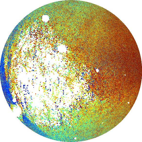
imprints great circles into the depth map. In Figure 2 we of α, δ, GBP − GRP , G, µα , µδ .
show the result of applying an unsharp-mask to all data at
Galactic latitudes |b| > 10◦ and with G < 20. A large num-
ber of stripy residuals can be seen, which could in principle
masquerade as streams. Any structures following this pat- 4 STREAMFINDER ANALYSIS
tern are almost certainly artefacts.
The STREAMFINDER algorithm is built to detect dynamically
cold and narrow tidal stellar streams that are possible rem-
1 These extinction ratios are listed on the Padova model site nants of globular clusters or very low-mass galaxies. At the
http://stev.oapd.inaf.it/cgi-bin/cmd 2.8. position of every star in the dataset, the algorithm finds the
MNRAS 000, 1–15 (2018)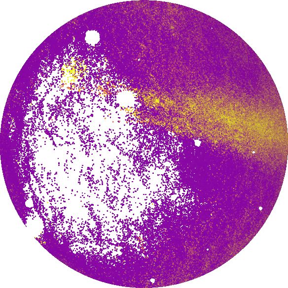
Stellar Streams in Gaia DR2                                3

                                       270°                                                                 90°
          N                                                                   S                                    X
                                                                                                                       PS1-C                  Dgal(kpc)
                                                                                                                                                     100

                225°                                   315°                       135°                                             45°
                                                                                                            PiscesOv
                                                                                                             X                                       80

                                                                                                                                     Sgr
                                                                                                                                          X          60

        180°                                                         0°   180°                                                                0°
                                                             Pal-5
                           GD-1        75                    X                                              -75    JhelumX                           40
                           X
                                   60                                                    X Eridanus    -60                     X
                                                                                                                         Indus                       20
                                  45          X                                                       -45
                135°                          Hermus   45°                        225°                                             315°
                                                                                                                                                     0
                                       90°                                                                  270°
Figure 1. Schematic stellar Stream map of the Milky Way sky prior to Gaia DR2. Here we show the Milky Way stellar stream map
(minus some stellar clouds) from the GALSTREAMS package (Mateu et al. 2018), transformed into polar ZEA projections. The colour
represents the Galacto-centric distances to these structures. The left and right panels show, respectively, the projection from the North
and South Galactic poles. The names of a few streams are labelled to help the reader’s orientation in this coordinate system. Galactic
longitude increases clockwise in the north panel and counter-clockwise in the south panel, while Galactic latitude changes radially as
shown.

                N                                                         S

Figure 2. Unsharp-mask map of the |b| > 10◦ sky, derived using Gaia sources brighter than G0 = 20. This simple filtering procedure
highlights the stripy artefacts that arise due to the inhomogeneous scanning of the sky in the DR2 catalogue. The same ZEA projections
are used here as in Figure 1. To create this map, we binned the catalogue into pixels of size 50.3 × 50.3, and subtracted from this the same
map but smoothed with a two-dimensional Gaussian of standard deviation 530 . The holes seen in the image correspond to the excised
regions around known clusters and satellite galaxies that were omitted in our analysis.

most likely stream model given the observed phase-space in-               (see Paper I for detailed discussion on the workings of the
formation, and quantifies the likelihood of that stream model             algorithm).
given the pre-calculated contamination model. To build the
                                                                               We used the STREAMFINDER to analyse the Gaia DR2
stream model, the algorithm launches orbits from the sky
                                                                          data in a similar way to that described in Paper I. The
position of the star in question, sampling over the proper
                                                                          orbits are integrated within the Galactic potential model
motion uncertainties, and over the full range of radial ve-
                                                                          1 of Dehnen & Binney (1998), and these orbits are then
locity. All possible distances to the star are examined that
                                                                          projected into the heliocentric frame of observables for com-
are consistent with the observed photometry and the chosen
                                                                          parison with the data. For this coordinate transformation,
stellar populations template. A by-product of the algorithm
                                                                          we assume a Galactocentric distance of the Sun of 8.20 kpc
is the orbital solution of every star along which stream lies
                                                                          (Karim & Mamajek 2017), a circular velocity Vcirc =

MNRAS 000, 1–15 (2018)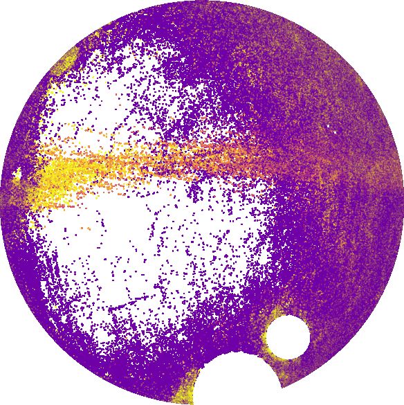
4     Malhan, Ibata & Martin
240 km s−1 and in addition we adopt the Sun’s peculiar ve-         lnLmax /lnLη=0 likelihood ratio is calculated for every star
locity to be V = (u , v , w ) = (9.0, 15.2, 7.0) km s−1            in the (filtered) catalogue, yet in the maps presented here
(Reid et al. 2014; Schönrich et al. 2010). As explained in        we only show those stars where this value exceeds 15. Many
Paper I, STREAMFINDER uses pre-selected isochrone models           other neighbouring stars may partake in a given stream
in order to sample orbits in distance space. The selected          structure, contributing to the high lnLmax /lnLη=0 valued-
isochrone model(s) essentially correspond to the proposed          points marked in the figure, yet they may not themselves
Single Stellar Population (SSP) model of the stream. Here,         pass the criterion and so are not shown. A given stream-like
we chose to work with Padova SSP models (Marigo et al.             structure seen in the figure is thus composed of many > 5σ
2008) in the Gaia photometric system, with age 10 Gyr              points. However, the points are not statistically indepen-
and with 7 metallicity values between [Fe/H] = −2.2 to             dent, as by construction information is correlated over the
[Fe/H] = −1.0 (spaced at 0.2 dex intervals). These isochrone       chosen 10◦ trial stream length. We further stress that the
models cover plausible values for Milky Way halo globular          aim of the STREAMFINDER algorithm is to enable the detec-
clusters (from which stellar streams are ultimately derived)2 .    tion of streams; a complete characterization and statistical
The candidate model streams were selected to have a Gaus-          analysis of a given detection should be accomplished with
sian width of 100 pc, and to be 10◦ long on the sky. Other         other tools, for instance, by careful modelling with N-body
parameter ranges used to integrate orbits in the Galaxy were       simulations.
identical to those detailed in Paper I.                                 The left and right panels of Figure 3 show, respectively,
     In Paper 1, our analysis was restricted to a small and        the projection from the North and South poles. The dis-
relatively high latitude patch of sky (∼ 100 deg2 ) in which       tance solutions displayed here are the ones obtained by the
the background stellar distribution (the halo) could be ap-        algorithm and span the inner halo range D = [5, 15] kpc.
proximated as a uniform distribution. In the present case,         The most visible feature in the northern hemisphere is the
where we are analysing vast regions of sky that have a non-        GD-1 stellar stream (Grillmair & Dionatos 2006; de Boer
uniform stellar distribution, it is important to consider the      et al. 2018), which appears as a > 60◦ stream in these spa-
background model of the Galaxy. Therefore, in contrast to          tial density maps of candidate stream members. It is pos-
Paper I, the likelihood function that we use here takes the        sible that it continues to lower Galactic latitude, where we
Galaxy into consideration via the smooth contamination             have not yet run the algorithm. Other notable detections are
model discussed above. Our log-likelihood function is sim-         the Jhelum and Indus streams (Shipp et al. 2018) seen in
ply:                                                               the Southern hemisphere in the more metal-poor map. As
       X                                                           a demonstration of the power of the algorithm, we display
lnL =       ln (ηPsignal (θ) + (1 − η) Pcontamination ) ,  (1)     the properties of GD-1, Jhelum and Indus, as recovered by
       data
                                                                   the STREAMFINDER, in Figure 4. Note that the distance so-
where θ are the stream fitting parameters, Pcontamination is       lutions to these streams that we obtain from STREAMFINDER
the probability density function of the smooth contamina-          match closely the distance values that have been previously
tion model that we obtain as explained in Section 3, and η         derived for these streams (as explained in Figure 4). The
is the fraction of the stream model compared to the con-           scatter in the distance solutions that is notably seen for in-
tamination. The adopted stream probability density func-           dividual streams could be a combination of the true intrinsic
tion Psignal is extremely simple: we take the trial orbit un-      dispersion of the stream and errors from mismatches with
der consideration and make it fuzzy by convolving it with          the isochrone template model (from which the distance so-
a Gaussian in each observed dimension. The Gaussian dis-           lutions are derived, see Paper I). We summarize some of
persions are: σsky representing the thickness of the stream,       the properties of these structures in Table 1, providing, for
σµα , σµδ representing the dispersions in proper motion, and       the first time, the proper motion values for the Jhelum and
σDM representing the dispersion in distance modulus (and           Indus streams.
hence in photometry). All these dispersions are the convolu-            The recovery of known stellar streams provides valida-
tion of the intrinsic Gaussian dispersion of the stream model      tion of our algorithm. Many other stream-like features can
together with the observational uncertainty on each star in        also be seen in this map, but these structures require de-
the Gaia DR2 catalogue.                                            tailed kinematic analysis for their confirmation (which is
                                                                   beyond of the scope of this paper). In the present contri-
                                                                   bution we will discuss the most obvious stream structures
5   RESULTS                                                        that not only have coherent phase-space properties (consis-
                                                                   tent with the template model and the data uncertainties)
In Figure 3 we show, for two representative metallicity
                                                                   but that also stand out significantly from the background.
values, the spatial distribution of the stars in the pro-
                                                                   These new streams, that are named Gaia-1,2,3,4, are shaded
cessed sample that have a high-likelihood of belonging
                                                                   in grey in Figure 3 and their phase-space properties are pre-
to a stream structure. These data are selected as having
                                                                   sented in Figure 9.
lnLmax /lnLη=0 > 15, where Lη=0 is the model likelihood
                                                                        Figure 5 shows the results at intermediate distances in
when no stream is present, and Lmax is the maximum like-
                                                                   the halo in the range D = [15, 30] kpc (again selecting
lihood stream solution found by the algorithm. Thus, our
                                                                   lnLmax /lnLη=0 > 15). Unlike Figure 3 that exhibits clearly
criterion corresponds to > 5σ when the noise distribu-
                                                                   distinguishable stream-like strings of stars, these maps pro-
tions are Gaussian. We would like to point out that the
                                                                   duced at intermediate distances are rather fuzzy and only
                                                                   seldom show thin stream-like features. Some of these stream
2 In subsequent papers, we plan to run the algorithm over a fine   features become apparent in the regions |b| > 45◦ where
grid in metallicity and age.                                       the density of contaminating stars is low. The most obvious

                                                                                                       MNRAS 000, 1–15 (2018)
Stellar Streams in Gaia DR2                  5

                                  270°                Age=10.0 , [Fe/H]=-1.0                         90°
           N                                                               S                                                D (kpc)
               225°                                 315°                        135°                                 45°
                                               Gaia-1
                                                                                                                                      14
                                                                                                   Gaia-2
                      GD-1
        180°                                                 0°         180°                                                 0°
                                75                                                                 -75
                           60                                                                -60
                      45                                                               -45
                                                                                                                                      12

               135°                                 45°                         225°                                315°
                                  90°                                                                270°
                                                      Age=10.0 , [Fe/H]=-1.6                                                          10
                                  270°                                                               90°
           N                               Gaia-3                          S
               225°                                 315°                        135°                                 45°
                            Gaia-4
                                                                                                                                      8
                      GD-1
        180°                                                 0°         180°                                                 0°
                                                                                                    Jhelum                            6
                                                                                                       Indus
               135°                                 45°                         225°                                315°
                                     90°                                                             270°
Figure 3. Potential stream stars identified by STREAMFINDER in the inner halo, from 5 to 15 kpc, in the same projection as Figure 1. The
colour represents the distance solutions that are obtained as a by-product for these stars from the STREAMFNIDER analysis. The top panels
show a metal-rich selection, while the lower panels show the results for intermediate metallicity. The most striking structure detected in
this distance range is the GD-1 stream (Grillmair & Dionatos 2006), seen clearly towards the lower end of the distance range (coloured
purple) in the Northern hemisphere (left panels). Several other streams are visible, including the Jhelum and Indus streams discovered
in the DES (Shipp et al. 2018). All stream points displayed here have detection significance > 5σ. New high confidence stream detections
are marked on the map, while the others will require confirmation with radial velocity measurements.

stream structure is Gaia-5, which is shaded in the grey circle          short arc of length ∼ 10◦ of the ∼ 60◦ long Orphan stream
in Figure 5 and its phase-space properties are presented in             (Grillmair 2006) in our outer halo spatial maps (again, the
Figure 9.                                                               chosen stream width of the model was not an appropriate
     The outer halo distribution, beyond 25 kpc is displayed            template for this structure, which may explain why the full
in Figure 6 (again selecting lnLmax /lnLη=0 > 15). The algo-            length was not recovered). For the position of the arc on
rithm highlights a veritable deluge of stream-like structures,          the sky shown in Figure 4, we find the distance solutions
which are seen over a range of distances and metallicities.             for the Orphan stream members to be compatible with the
Comparison to Figure 1 shows that we detect the Sagittar-               study by Newberg et al. (2010). Also, we find that its mem-
ius stream (Ibata et al. 2001; Majewski et al. 2003) over a             ber stars have a tight proper motion distribution (Table 1
large swathe of the outer halo. This is somewhat surprising,            provides proper motion values for the Orphan stream). This
since we set the stream model width to 100 pc, which is ap-             map also requires follow-up with radial velocity measure-
propriate for a globular cluster, but is actually a very poor           ments in order to test the phase-space consistency of the
template for this wide stream. We suspect that the spatial              other possible stream like structures that are distributed on
inhomogeneities in Gaia due its scanning law may partially              these maps (for example, see the bottom panels of Figure
explain the striated aspect of the Sagittarius stream in our            6).
maps (see, e.g., Figure 6). The algorithm also detected a                    Careful visual inspection of these maps indicated that

MNRAS 000, 1–15 (2018)
6 Malhan, Ibata & Martin
11 20
60 GD-1 [Fe/H]=-1.6 14 Age = 10Gyrs
10 10 [Fe/H] = -1.6
50
(mas yr 1)
(degrees)
9
D (kpc)
40 0 16
8
G
30 7 10
18
20 6 20
10 5
140 160 180 200 140 160 180 200 20 10 0 10 20 0.5 1.0
16 20
46 Jhelum [Fe/H]=-1.6 14 Age = 10Gyrs
15 10 [Fe/H] = -1.6
(mas yr 1)
48
(degrees)
14
D (kpc)
0 16
50 13
G
52 12 10
18
54 11 20
10
320 340 360 320 340 360 20 10 0 10 20 0.5 1.0
50 20 20
Indus [Fe/H]=-1.4 14 Age = 10Gyrs
19 10 [Fe/H] = -1.4
55
(mas yr 1)
(degrees)
18
D (kpc)
0 16
60 17
G
16 10
65 18
15 20
70 14
320 330 340 350 360 320 330 340 350 360 20 10 0 10 20 0.5 1.0
40 20
Orphan [Fe/H]=-2.0 14 Age = 10Gyrs
40 10 [Fe/H] = -2.0
38
(mas yr 1)
(degrees)
35
D (kpc)
0 16
36 G
30
10
25 34 18
20
20 32
145 150 155 145 150 155 20 10 0 10 20 0.5 1.0
(degrees) (degrees) * (mas yr 1) GBP GRP
Figure 4. Properties of a sample of previously-discovered streams, as recovered by the STREAMFINDER. The first, second, third and fourth
rows show the properties of the GD-1, Jhelum, Indus and Orphan streams, respectively. The columns reproduce, from left to right, the
equatorial coordinates of the structures, the distance solutions found by the algorithm (for representative metallicity values), the proper
motion distribution (with observations in red, model solutions in blue, and the full DR2 sample in grey), and the colour-magnitude
distribution of the stars (with observations in red and template model in blue) selected by STREAMFINDER. The distance solutions found
by the algorithm match closely the distance values that have been previously derived for these streams: D ∼ 8 kpc for GD-1 (Grillmair
& Dionatos 2006), D ∼ 13.2 kpc and ∼ 16.6 kpc for Jhelum and Indus, respectively (Shipp et al. 2018) and D = [33 − 38] kpc for
Orphan (Newberg et al. 2010). The CMD template models, shown in blue in the last column, have been plotted at the appropriate
distance for the respective streams. The colour-magnitude diagram of the Orphan stream might seem peculiar, but here we only see the
red-giant branch due to the trimming of the data sample below G = 19.5.
the stream-like structures recovered by the algorithm are not considerable more processing time to examine the necessary
associated with the extinction correction. In Figures 7 and parameter space), but rather to present a preview of the
8, we present our summary plots made by combining the dis- large-scale stream structure of our Galaxy. Nevertheless, we
tance and metallicity samples for the north and south hemi- have selected by hand a small number of structures that
spheres, respectively. The top panels of these diagrams show appear clearly in our maps, with kinematic properties that
the estimate of the distances of these structures (provided distinguish them from the contaminating Galactic popula-
by the algorithm), while the bottom panels show an esti- tion, and that are clearly not artefacts produced by Gaia’s
mate of the magnitude of the tangential velocity calculated scanning law. A large number of other stream candidates
using the measured Gaia proper motions combined with the have a clearly-defined stream-like morphology, but possess
distance estimates. Many structures are beautifully resolved proper motions distributions that are similar to that of the
in this multi-parameter space. halo, and we deem that they require further follow-up to be
Our aim in this contribution is not to present a thorough confident of their nature.
or complete census of halo streams (since it would require The locations of the five structures we selected are
MNRAS 000, 1–15 (2018)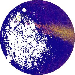
Stellar Streams in Gaia DR2               7

                                 270°                Age=10.0 , [Fe/H]=-1.2                        90°
           N                                                             S
               225°                                315°                       135°                                45°
                                                                                                                         D (kpc)
                                                                                                                                   30

        180°                                                0°        180°                                                0°
                                75                                                               -75
                           60                                                              -60                                     28
                      45                                                             -45

               135°                                 45°                       225°                               315°
                                 90°                                                               270°                            26

                                 270°                Age=10.0 , [Fe/H]=-1.6                        90°
           N                                                             S
               225°                                315°                       135°                                45°
                                                                                                                                   24

        180°                                                0°        180°                                                0°
                                                                                                                                   22

               135°                                 45°                       225°                               315°
                                                                                                                                   20
                                 90°                                                               270°
                                 270°                Age=10.0 , [Fe/H]=-2.2                        90°
           N                                                             S
               225°                                315°                       135°                                45°
                                                                                                                                   18

        180°                                                0°        180°                                                0°
                      Gaia-5                                                                                                       16

               135°                                 45°                       225°                               315°
                                     90°                                                           270°
Figure 5. Spatial distribution of stream candidates at intermediate distances. Here we show the stellar stream density map as obtained
from the STREAMFINDER based on 3 representative isochrone models. Each row corresponds to a particular isochrone model of age (in
Gyr) and metallicity, as labelled. The left panels represent the North side of the ZEA projection system and the right panels represent
the South. The colour scale is proportional to the heliocentric distances to the stellar members of the detected structures obtained as
a by-product from the STREAMFINDER analysis. All streams displayed here have detection significance > 5σ. New high confidence stream
detections are marked on the map.

MNRAS 000, 1–15 (2018)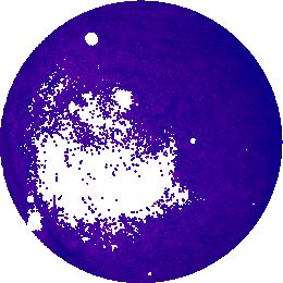
8     Malhan, Ibata & Martin

                                  270°                 Age=10.0 , [Fe/H]=-1.2                        90°
           N                                                               S
                225°                                 315°                       135°                                  45°
                                                                                                                              D (kpc)
                                                                                                                                        100

        180°                                                  0°         180°                                                 0°
                                 75                                                                -75
                            60                                                               -60                                        90
                       45                                                              -45

                135°                                  45°                       225°                                 315°
                                                                                                                                        80
                                  90°                                                                270°
                                  270°                 Age=10.0 , [Fe/H]=-1.6                        90°
           N                                                               S
                225°                                 315°                       135°                                  45°               70

        180°                                                  0°         180°                                                 0°        60

                135°                                  45°                       225°                                 315°               50

                                  90°                                                                270°
                                  270°                 Age=10.0 , [Fe/H]=-2.0                        90°
           N                                                               S                                                            40
                225°                                 315°                       135°                                  45°

                                                                                                                                        30
        180°                                                  0°         180°                                                 0°
                       Orphan

                                                                                                                                        20
                135°                                  45°                       225°                                 315°
                                      90°                                                            270°
Figure 6. As Figure 5, but for the outer halo beyond 25 kpc. The dominant structure seen out to large heliocentric distances in both
hemispheres is the Sagittarius stream, which is detected despite the narrowness of the stream template model that we set in our algorithm.
The interesting bifurcation of this structure is seen in the top-left panel. In addition, the lower-left panel shows an overdensity of stars
in the region where the Orphan stream lies (Grillmair 2006). Many other stream-like features are also detected, but most are confined
to the nearer limit of the distance range shown.

                                                                                                                MNRAS 000, 1–15 (2018)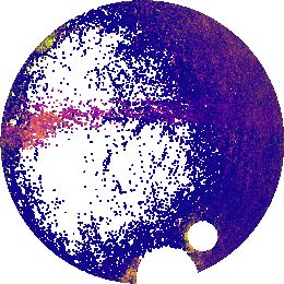
Stellar Streams in Gaia DR2                  9

                                                                  270°
                         GALACTIC SKY                                                                           D (kpc)
                         NORTH                                                                                           50

                                      225°                                                    315°

                                                                                                                         40

                                                                                                                         30
                          180°                                                                             0°
                                                           75
                                                   60                                                                    20
                                             45

                                                                                                                         10
                                      135°                                                     45°

                                                                  90°

                                                                  270°
                         GALACTIC SKY                                                                      VT (kms 500
                                                                                                                    1)
                         NORTH
                                      225°                                                    315°

                                                                                                                     400

                                                                                                                     300

                          180°                                                                             0°
                                                           75
                                                                                                                     200
                                                   60
                                             45

                                                                                                                     100

                                      135°                                                     45°

                                                                                                                     0

                                                                  90°

Figure 7. Summary diagrams of the distance (D > 5 kpc) and tangential velocity VT of stream-like structures in the northern Galactic
sky. The tangential velocities are calculated based on the observed proper motion of the stars in DR2 and the corresponding distance
estimates that we obtain from the algorithm. Most of the structures that we report here are visible in these diagrams, as are many others
that we intend to investigate further in future contributions.

MNRAS 000, 1–15 (2018)
10   Malhan, Ibata & Martin

                                                    90°
                GALACTIC SKY                                                               D (kpc)
                SOUTH                                                                               50

                        135°                                                   45°
                                                                                                    45

                                                                                                    40

                                                                                                    35

                                                                                                    30
                180°                                                                  0°
                                             75
                                                                                                    25
                                     60
                               45                                                                   20

                                                                                                    15

                        225°                                                   315°
                                                                                                    10

                                                   270°

                                                    90°
                GALACTIC SKY                                                          VT (kms 500
                                                                                               1)
                SOUTH
                        135°                                                   45°

                                                                                                400

                                                                                                300

                180°                                                                  0°
                                             75
                                                                                                200
                                     60
                               45

                                                                                                100

                        225°                                                   315°

                                                                                                0

                                                   270°

                         Figure 8. As Figure 7, but for the southern Galactic sky.

                                                                                           MNRAS 000, 1–15 (2018)
Stellar Streams in Gaia DR2 11
marked in Figures 3 and 5, and their properties are shown value of ∼ 0.36 mas yr−1 (and proper motion dispersion of
in Figure 9, and are also summarised in Table 1. All these ∼ 0.70 mas yr−1 ), the fact that it emerges as a highly co-
structures that we find have significance > 5σ. herent structure in our maps makes it a confident structure.
Here, we detect it as a very cold structure in proper motion
space.
5.1 Gaia-1
Gaia-1 has an angular extent of ∼ 15◦ and projected width
5.5 Gaia-5
of ∼ 0.5◦ . The orbital solutions provided by the algorithm
imply that it is situated at a distance of D ∼ 5.5 kpc, We include Gaia-5 here as another interesting detection
which is in reasonable agreement with the Gaia parallax (bottom row panels in Figure 9), as it is parallel to the GD-
measurement of 0.216 ± 0.038 mas (i.e. 4.6 kpc). This means 1 stream, and could easily have been confused with GD-1
that Gaia-1 has a physical width of ∼ 40 pc. The narrowness without Gaia’s excellent proper motion measurements. The
of the stream suggests that the progenitor likely is or was properties of this object are shown in red for positions, ob-
a globular cluster. Moreover, Gaia-1 has a strikingly high served proper motions and photometry, and in blue for dis-
proper motion value of ∼ 23.5 mas yr−1 , implying that it has tance and and proper motion orbital solutions. We also in-
a transverse motion ∼ >
500 km s−1 . It will be worthwhile to clude the properties of GD-1 (in green) for comparison. The
measure the radial velocity of this system, as it may provide proper motions, along with the distance solutions, of Gaia-
an interesting constraint on the Galactic potential simply 5 stars are distributed over a compact region that is very
from the requirement that the system is bound to the Milky far from the region inhabited by GD-1; also the two colour-
Way. magnitude distributions (CMDs) are very different and well
separated. Hence, unlike the possible bimodal stream distri-
bution that we recognise in Gaia-3, we identify Gaia-5 as a
5.2 Gaia-2 stream unrelated to GD-1. The (error-weighted mean) par-
Gaia-2 turns out to be a considerably thin structure in our allax value we calculate for this structure would imply that
spatial maps. Extending over ∼ 10◦ in length, we find that it is substantially closer to the Sun than GD-1, which is
it possesses a distance gradient ranging from D = [10– both inconsistent with the model solutions of ∼ 20 kpc, and
13] kpc. Given its narrowness and the location in the halo, is very difficult to reconcile with the CMD. However, our
we also suspect it to be a remnant of a globular clus- simple combination of the parallax measurements is highly
ter. We find Gaia-2 to be a highly coherent structure in susceptible to contaminants, which may explain the incon-
proper motion space with an average proper motion mag- sistency.
nitude of ∼ 6.5 mas yr−1 and proper motion dispersion of We plan to examine these structures (and the many
∼ 0.75 mas yr−1 . other stream candidates visible in Figures 7 and 8) in de-
tail in later contributions. Careful analysis based on their as-
trometry and photometry, along with the mapping of these
5.3 Gaia-3 structures in deeper astrophysical catalogues (e.g. SDSS,
PS1, DES), would render a fuller insight into their origin,
Gaia-3 can be easily identified as an isolated stream struc-
orbits and phase-space distribution. Some of the previously-
ture in Figure 3. In Figure 9 (third row), Gaia-3 clearly
known streams and new detections appear to present spatial
shows two distinct possible sets of distance solutions. The
kinks, which is probably the effect of low-number statistics.
separation of these two different sets of solutions in position,
distance and colour-magnitude distribution space, while not
so much in proper motion space, suggests that what we de-
tect here as Gaia-3 might in fact be a superposition of two 6 DISCUSSIONS AND CONCLUSIONS
streams, or a more complicated structure aligned along the In this contribution, we present a new stellar stream map
line of sight. We shall describe this structure collectively of the Milky Way halo, obtained by the application of our
here. STREAMFINDER algorithm (described in Paper I) on the re-
Gaia-3 is found to be extended over ∼ 16◦ in sky with cently published ESA/Gaia DR2 catalogue. This is the first
a distance range of D = [9–14 kpc] with an average proper time an all-sky structural and kinematic map of the stel-
motion magnitude of ∼ 7.4 mas yr−1 . Given its peculiar- lar streams of the Milky Way halo has been constructed.
ity, as suggested above and shown in Figure 9, it is hard Our algorithm detects numerous previously-known streams,
to comment on its physical width or the progenitor. The which were discovered in much deeper photometric datasets
distance estimate of this structure too was found to be (e.g. SDSS, PS1, DES), confirming that our method, which
in good agreement with the Gaia parallax measurement of includes proper motion information, works as designed. In-
0.101 ± 0.013 mas (i.e. 9.8 kpc). deed, the fidelity of the GD-1 detection is striking, and re-
veals that the excellent Gaia proper motions provide very
powerful discrimination.
5.4 Gaia-4
In addition, we find a large number of streams and
Gaia-4 appears to be a fine linear structure, found at a dis- stream candidates throughout the distance range probed. In
tance of ∼ D = 11 kpc. Given its narrowness and dis- this first exploration, we selected five good streams (named
tance, we suspect the progenitor to be a globular clus- here as Gaia-1,2,3,4,5), to showcase the results, but many
ter. Although we find Gaia-4 sitting within the range of other candidates will require careful follow-up. In particular,
halo field stars in proper motion space with an average the fact that Gaia scans the sky along great circles, but with
MNRAS 000, 1–15 (2018)12 Malhan, Ibata & Martin
0 9 20
Gaia-1 8
[Fe/H]=-1.0 14
5 10
(mas yr 1)
(degrees)
7
D (kpc)
0 16
10 6
G
5 10
15 18
4 20
20 3
180 185 190 195 200 180 185 190 195 200 20 10 0 10 20 0.5 1.0
18 14 20
20
Gaia-2 13
[Fe/H]=-1.0 14
10
(mas yr 1)
(degrees)
22 12
D (kpc)
0 16
24 11
G
26 10 10
18
28 9 20
30 8
5 10 15 5 10 15 20 10 0 10 20 0.5 1.0
15 20
10 Gaia-3 [Fe/H]=-1.6 14
14 10
15
(mas yr 1)
(degrees)
13
D (kpc)
20 0 16
12
G
25
11 10
30 18
10 20
35
9
172 174 176 178 172 174 176 178 20 10 0 10 20 0.5 1.0
2 15 20
4
Gaia-4 14
[Fe/H]=-1.6 14
10
(mas yr 1)
(degrees)
6 13
D (kpc)
0 16
8 12 G
10 11 10
18
12 10 20
14 9
162 164 166 168 162 164 166 168 20 10 0 10 20 0.5 1.0
45 25 20
Gaia-5 [Fe/H]=-2.0 14
40 20 10
(mas yr 1)
(degrees)
D (kpc)
35 0 16
15
G
30 10
10 18
25 20
135 140 145 150 155 135 140 145 150 155 20 10 0 10 20 0.5 1.0
(degrees) (degrees) * (mas yr 1) GBP GRP
Figure 9. As Figure 4 but for the selected set of newly-discovered streams. Oddly, for Gaia-3, we found two distinct possible sets of
solutions based on distance estimates that we obtained from our algorithm, as highlighted in the respective panel. The more distant stars
are coloured in green, while the relatively nearby ones are shown in red. This clear distinction of these two different sets of solutions in
position, distance and colour-magnitude distribution space, while not so much in proper motion space, suggests that what we detect here
as Gaia-3 might in fact be a superposition of two streams, or a more complicated structure aligned along the line of sight. The bottom
row shows the properties of Gaia-5, which is found to lie parallel, but slightly offset, to GD-1 (shown on this bottom row in green).
Nevertheless, it is very distinct from GD-1 both in its proper motion distribution and in its colour-magnitude distribution.
an inhomogeneous number of visits, causes density inhomo- the survey noise properties very complex, invalidating the
geneities that appear like great circle streaks on the sky. This assumptions behind our lnLmax /lnLη=0 > 15 selection cri-
could cause some spurious stream detections (although the terion. This means, unfortunately, that the effective stream
kinematics test in the STREAMFINDER algorithm should allow detection threshold is not uniform in our sky maps, and the
us to reject most such fake streams). Nevertheless, these significance of the detections is lower in regions where the
spatial inhomogeneities in the Gaia DR2 necessarily make Gaia inhomogeneities are more pronounced.
MNRAS 000, 1–15 (2018)Stellar Streams in Gaia DR2 13
Table 1. Parameters of the stellar streams. The “Position” column gives the extent of these structures, ‘D ’ is the approximate range of
the distance solution as obtained by our algorithm, while column 4 lists the range of observed proper motion of the structure in the 2D
proper motion space. The parallax π is an uncertainty-weighted average of the Gaia measurements; for those objects where the parallax
uncertainty is less than 33% of the parallax, we also provide the corresponding distance. The discrepancy between the model distances
and mean parallax measurement for the cases of Indus and Gaia-5 may be due to contaminants in the samples affecting the simple
weighted average parallax reported here.
1
Name Position D (model) (µ∗α , µδ ) π
π
(extent) ( kpc) ( mas yr−1 ) (mas) ( kpc)
GD-1 135◦14 Malhan, Ibata & Martin
predicted STREAMFINDER radial velocities to probe the orbital National Cosmology et Galaxies (PNCG) of CNRS/INSU
properties of the stellar stream population as a whole. with INP and IN2P3, co-funded by CEA and CNES. N.
Several more streams have been reported within 40 kpc F. Martin gratefully acknowledges the Kavli Institute for
than the five that we recover here (see Figure 1). The rea- Theoretical Physics in Santa Barbara and the organizers of
son for this is likely to be due, in part, to the specific pa- the “Cold Dark Matter 2018” program, during which some
rameter choices we adopted in the algorithm (for instance of this work was performed. This research was supported in
we chose a model width of 100 pc throughout, and we ex- part by the National Science Foundation under Grant No.
amined only a narrow range of stellar population template NSF PHY11-25915
models). In subsequent contributions, we intend to relax
these constraints allowing for a more complete census to
be established. Additionally, we intend to examine different
models of the Galactic potential; presumably our stream de- REFERENCES
tection method should reveal the highest contrast for long
stellar streams when using the correct potential. However, Balbinot E., Gieles M., 2018, MNRAS, 474, 2479
Belokurov V., et al., 2006, ApJ, 642, L137
another reason that we did not recover all known streams
Bernard E. J., et al., 2014, MNRAS, 443, L84
within 40 kpc is simply that Gaia’s photometry is not as
Bonaca A., Hogg D. W., 2018, preprint, (arXiv:1804.06854)
deep as existing sky surveys; note that for a stellar popu- Bovy J., 2016, Physical Review Letters, 116, 121301
lation of metallicity [Fe/H] = −1.5, the distance at which Bovy J., Bahmanyar A., Fritz T. K., Kallivayalil N., 2016, ApJ,
the proper motion uncertainties in Gaia DR2 at the main 833, 31
sequence turnoff are 50 km s−1 (i.e. approximately half the Bullock J. S., Boylan-Kolchin M., 2017, ARA&A, 55, 343
dispersion of the contaminating halo) is 14.0 kpc. Hence it is Carlberg R. G., Grillmair C. J., Hetherington N., 2012, ApJ, 760,
not very surprising that photometric surveys that are much 75
deeper than Gaia remain competitive for finding low-mass Dehnen W., Binney J., 1998, MNRAS, 294, 429
stellar streams at distances ∼ >
15 kpc. Erkal D., Belokurov V., Bovy J., Sanders J. L., 2016, MNRAS,
Thanks to the amazingly rich phase-space information 463, 102
Evans, D. W. et al., 2018, A&A
provided by the Gaia spacecraft and consortium, we are now
Eyre A., Binney J., 2009, MNRAS, 400, 548
starting to unravel the very fine details of galaxy forma-
Gaia Collaboration et al., 2016, A&A, 595, A2
tion in action. While the results presented here are but a Gaia Collaboration Brown, A. G. A. Vallenari, A. Prusti, T. de
first step in the comprehensive mapping of the Milky Way’s Bruijne, J. H. J. et al. 2018, A&A
stellar halo and accretion events, they already show the Grillmair C. J., 2006, ApJ, 645, L37
promises borne out by the deep, multi-dimensional space Grillmair C. J., Carlin J. L., 2016, in Newberg H. J., Car-
unveiled in DR2. The harvest of previously unknown thin lin J. L., eds, Astrophysics and Space Science Library Vol.
stellar streams, likely stemming from the tidal disruption of 420, Tidal Streams in the Local Group and Beyond. p. 87
globular clusters, opens up exciting times as these are pow- (arXiv:1603.08936), doi:10.1007/978-3-319-19336-6˙4
erful probes of the distribution of dark matter sub-halos in Grillmair C. J., Dionatos O., 2006, ApJ, 643, L17
our surroundings (Johnston et al. 2002; Ibata et al. 2002; Harris W. E., 2010, preprint, (arXiv:1012.3224)
Helmi A., White S. D. M., 1999, in Gibson B. K., Axelrod R. S.,
Carlberg et al. 2012; Bovy 2016), they can provide an inde-
Putman M. E., eds, Astronomical Society of the Pacific Con-
pendent inference of the location of the Sun in phase space ference Series Vol. 165, The Third Stromlo Symposium: The
(Malhan & Ibata 2017), and they can be used as sensitive Galactic Halo. p. 89 (arXiv:astro-ph/9811108)
seismographs to constrain the shape and depth of the Milky Helmi, A. van Leeuwen, F. McMillan, P. DPAC 2018, A&A
Way potential (Ibata et al. 2013; Bonaca & Hogg 2018). Ibata R., Lewis G. F., Irwin M., Totten E., Quinn T., 2001, ApJ,
The combination of Gaia DR2 and detections provided by 551, 294
STREAMFINDER places us in a unique position to disentan- Ibata R. A., Lewis G. F., Irwin M. J., Quinn T., 2002, Monthly
gle the numerous detections accretion events in the Milky Notices of the Royal Astronomical Society, 332, 915
Way halo and open the most exciting Galactic archaeology Ibata R., Lewis G. F., Martin N. F., Bellazzini M., Correnti M.,
playground to date. 2013, ApJ, 765, L15
Ibata R. A., et al., 2017a, ApJ, 848, 128
Ibata R. A., et al., 2017b, ApJ, 848, 129
Ibata R. A., Malhan K., Martin N. F., Starkenburg E., 2018,
ACKNOWLEDGEMENTS preprint, (arXiv:1806.01195)
Johnston K. V., Hernquist L., Bolte M., 1996, ApJ, 465, 278
We thank the anonymous referee very much for their helpful Johnston K. V., Zhao H., Spergel D. N., Hernquist L., 1999, ApJ,
comments. 512, L109
This work has made use of data from the European Johnston K. V., Spergel D. N., Haydn C., 2002, ApJ, 570, 656
Space Agency (ESA) mission Gaia (https://www.cosmos. Karim M. T., Mamajek E. E., 2017, MNRAS, 465, 472
esa.int/gaia), processed by the Gaia Data Processing and Koposov S. E., Rix H.-W., Hogg D. W., 2010, ApJ, 712, 260
Küpper A. H. W., Balbinot E., Bonaca A., Johnston K. V., Hogg
Analysis Consortium (DPAC, https://www.cosmos.esa.int/
D. W., Kroupa P., Santiago B. X., 2015, ApJ, 803, 80
web/gaia/dpac/consortium). Funding for the DPAC has
LSST Dark Energy Science Collaboration 2012, preprint,
been provided by national institutions, in particular the in- (arXiv:1211.0310)
stitutions participating in the Gaia Multilateral Agreement. Law D. R., Majewski S. R., 2010, ApJ, 714, 229
The authors would like to thank Michel Ringenbach of Lindegren, L. Hernandez, J. Bombrun, A. Klioner, S. Bastian, U.
the HPC centre of the Université de Strasbourg for his kind Ramos-Lerate, M. 2018, A&A
support. We also acknowledge support by the Programme Luri, Xavier et al., 2018, A&A
MNRAS 000, 1–15 (2018)Stellar Streams in Gaia DR2 15 Majewski S. R., Skrutskie M. F., Weinberg M. D., Ostheimer J. C., 2003, ApJ, 599, 1082 Malhan K., Ibata R. A., 2017, MNRAS, 471, 1005 Malhan K., Ibata R. A., 2018, MNRAS, Marigo P., Girardi L., Bressan A., Groenewegen M. A. T., Silva L., Granato G. L., 2008, A&A, 482, 883 Mateu C., Read J. I., Kawata D., 2018, MNRAS, 474, 4112 McConnachie A. W., 2012, AJ, 144, 4 Newberg H. J., Willett B. A., Yanny B., Xu Y., 2010, ApJ, 711, 32 Reid M. J., et al., 2014, ApJ, 783, 130 Robin A. C., et al., 2012, A&A, 543, A100 Sanders J. L., Bovy J., Erkal D., 2016, MNRAS, 457, 3817 Sanderson C., Curtin R., 2017, Journal of Open Source Software, 2 Schlegel D. J., Finkbeiner D. P., Davis M., 1998, ApJ, 500, 525 Schönrich R., Binney J., Dehnen W., 2010, MNRAS, 403, 1829 Shipp N., et al., 2018, preprint, (arXiv:1801.03097) de Boer T. J. L., Belokurov V., Koposov S. E., Ferrarese L., Erkal D., Cote P., Navarro J. F., 2018, preprint, (arXiv:1801.08948) de Bruijne J. H. J., 2012, Ap&SS, 341, 31 This paper has been typeset from a TEX/LATEX file prepared by the author. MNRAS 000, 1–15 (2018)
You can also read