Combined Peridynamics and Discrete Multiphysics to Study the Effects of Air Voids and Freeze-Thaw on the Mechanical Properties of Asphalt - MDPI

Article

Combined Peridynamics and Discrete Multiphysics to Study
the Effects of Air Voids and Freeze-Thaw on the Mechanical
Properties of Asphalt
Danilo Sanfilippo 1,2, Bahman Ghiassi 1,*, Alessio Alexiadis 2,* and Alvaro Garcia Hernandez 1,*

 1 Department of Civil Engineering, University of Nottingham, NG7 2RD, Nottingham, UK;
 danilo.sanfilippo@nottingham.ac.uk
 2 School of Chemical Engineering, University of Birmingham, B15 2TT, Birmingham, UK

 * Correspondence: bahman.ghiassi@nottingham.ac.uk (B.G.); alvaro.garcia@nottingham.ac.uk (A.A.);
 A.Alexiadis@bham.ac.uk (A.G.H.)

 Abstract: This paper demonstrates the use of peridynamics and discrete multiphysics to assess mi-
 cro crack formation and propagation in asphalt at low temperatures and under freezing conditions.
 Three scenarios are investigated: (a) asphalt without air voids under compressive load, (b) asphalt
 with air voids and (c) voids filled with freezing water. The first two are computed with Peridynam-
 ics, the third with peridynamics combined with discrete multiphysics. The results show that the
 presence of voids changes the way cracks propagate in the material. In asphalt without voids, cracks
 tend to propagate at the interface between the mastic and the aggregate. In the presence of voids,
Citation: Sanfilipo, D.; Bahman, G.; they ‘jump’ from one void to the closest void. Water expansion is modelled by coupling Peridynam-
Alexiadis, A.; Hernandez Garcia, A. ics with repulsive forces in the context of Discrete Multiphysics. Freezing water expands against the
Combined Peridynamics and
 voids’ internal surface, building tension in the material. A network of cracks forms in the asphalt,
Discrete Multiphysics to Study the
 weakening its mechanical properties. The proposed methodology provides a computational tool for
Effects of Air Voids and
 generating samples of ‘digital asphalt’ that can be tested to assess the asphalt properties under dif-
Freeze-thawon the Mechanical
 ferent operating conditions.
Proper-Ties of Asphalt. Materials
2021, 14, 1579. https://doi.org/
10.3390/ma14071579
 Keywords: asphalt; mathematical modelling; peridynamics; discrete multiphysics

Academic Editors: Gilda Ferrotti and
Francesco Canestrari
 1. Introduction
Received: 28 December 2020 Asphalt, a heterogeneous mixture of aggregates, fillers and asphalt binder, is one of
Accepted: 16 March 2021
 the most used infrastructure material. Asphalt’s mechanical properties are influenced by
Published: 24 March 2021
 the properties of its constituents, its internal structure and the loading and environmental
 conditions during its service life. Understanding the degradation of asphalt, such as rut-
Publisher’s Note: MDPI stays neu-
 ting, ravelling, freezing, strength loss and fatigue cracking, is important for better design,
tral with regard to jurisdictional
claims in published maps and institu-
 manufacture and maintenance of roads.
tional affiliations.
 One of the major sources of deterioration of asphalt is cracking. The fracture process
 can be divided into two different stages [1,2]: crack initiation and propagation. Crack ini-
 tiation occurs when the mechanical stress is higher than a given limit, and micro-cracks
 occur in the mastic [3]. Under continuous load, these micro-cracks coalesce into macro-
Copyright: © 2021 by the authors. Li- cracks, which initiate the propagation phase that ultimately, leads to failure [1]. The
censee MDPI, Basel, Switzerland. growth of microcracks damages asphalt irreversibly and increases maintenance costs [4],
This article is an open access article and this is influenced by different factors such as temperature, loading level and rate,
distributed under the terms and con- fatigue and mixture composition.
ditions of the Creative Commons At- Another cause of asphalt failure in cold regions is thermal cracking (at low tempera-
tribution (CC BY) license (http://crea- tures), which may significantly reduce the durability of pavements [5,6]. This damage is
tivecommons.org/licenses/by/4.0/). especially severe when water is present in the asphalt pores due to its comparatively high
 thermal expansion. Under icing temperatures, the internal pore structure in an asphalt

Materials 2021, 14, 1579. https://doi.org/10.3390/ma14071579 www.mdpi.com/journal/materials

Materials 2021, 14, 1579 2 of 19

 mixture may change following a three-stage process [7]: (i) water expansion, which causes
 damage, and expansion of the exiting pores; at −10 °C, for instance, water undergoes 15%
 volume expansion [8]; (ii) cracking and merging of the pores and (iii) creation of new voids
 [9]. This phenomenon is especially intense in asphalts with a porosity between 6% and
 13%, which retain part of the pore water. Asphalts with 13% voids have large pores that do not
 retain water [10–12].
 There are many studies, both theoretical and experimental, on asphalt degradation
 (e.g., [3,4,13–16]), but only a few experimental works dedicated to low temperatures and
 freeze-thawcycles [5–7,17–19]. Furthermore, the experimental tests cannot show the evo-
 lution of the damage inside the asphalt’s microstructure, which is critical for understand-
 ing the deterioration mechanisms. To the best of our knowledge, there are also no availa-
 ble numerical methods for predicting degradation of asphalt or monitoring the damage
 progression resulting from freeze-thawactions. The development of such modelling tools,
 the subject of this paper, allows estimation of asphalt’s service life performance under cold
 environmental conditions. This is critical for optimising asphalt or developing novel ma-
 terials with enhanced durability and long-term performance.
 Recent advancements in computer technology allow performing realistic simulations
 of the performance of materials across scales. Novel mesh-free methods are more suited
 for this purpose as they allow simulation of crack propagation and branching without the
 need for mesh regeneration. One of the simplest mesh-free methods is the lattice spring
 model (LSM) that divides solids into computational particles linked together with springs
 [20–22]. Peridynamics (PD) [23] is a novel mesh-free method developed as an improve-
 ment of the LSM [24] to allow better simulation of the material damage response. The
 application of PD to the simulation of damage in construction materials is highly innova-
 tive and limited, and its asphalt application will be presented in this paper for the first
 time.
 This paper aims to develop a computational tool that allows realistic simulation of
 the damage of asphalt under mechanical and freeze-thawloads. We present a PD model
 coupled with discrete multiphysics developed in the LAMMPS molecular dynamics sim-
 ulation package. This requires developing realistic models considering the aggregates and
 binder, voids and water, both in liquid and solid forms. Optical and micro-CT images are
 used to develop models considering the internal microstructure of a range of asphalt ma-
 terials. PD implemented in LAMMPS also allows considering the plastic [25] and viscoe-
 lastic [26] response of materials and is therefore suitable for simulation of the response of
 asphalt materials under higher temperatures. The state-based Peridynamics is used here
 to evaluate the mechanical response of intact asphalt before and after being subjected to a
 freeze-thawcycle. The internal damage in the asphalt due to freezing is simulated by cou-
 pling Peridynamics with repulsive forces obtained from expansion of liquid phases and
 their transformation into solid phase using Discrete Multiphysics (DMP) [27–29]. The
 model is then used to discuss the effect of the freezing of the water present in the voids
 on the asphalt’s mechanical response.

 2. Theory
 2.1. Peridynamics
 In Peridynamics, the material’s body is defined as a lattice, and contrary to classical
 continuum mechanics, its behaviour is defined through a constitutive equation that links
 deformation and force rather than strain and stress. The original bond-based Peridynamic
 approach [23] was limited to materials with a Poisson ratio ¼ in 3D and ⅓ in 2D. State-
 based Peridynamics [30] was introduced to overcome these limitations. In state-based
 Peridynamics, the forces that connect two bonded elements depend on the overall state of
 all the particles located within a material horizon rather than the single bond. The accel-
 eration of any particle at position x in the reference configuration at time t is found from:

Materials 2021, 14, 1579 3 of 19

 ρ( )ü( , t) = T ( , t)⟨ − ⟩ − T( , t)⟨ − ′⟩ dV′ + ( , t) (1)

 where ρ(x) is the mass density at x, u is the displacement vector field, Hx is a neighborhood
 of with radius containing all the points ′ within the horizon, T ( , )⟨ − ⟩ is the
 pairwise force state function at time t whose value is the force vector (per unit volume
 squared) acting between two particles within the horizon applied to the bond ⟨ − ⟩,
 dV′ is the infinitesimal volume, b is a body force density field. The relative position vector
 state of these two particles in the reference configuration ε is given by
 ⟨ ’ − ⟩ = ’ − = (2)

 where X represents the reference state, mapping all bonds in a non-deformed body, B0.
 The relative displacement vector state U is associated with the bond by:
 ⟨ − ⟩ = u( ′, t) − u( , t) = (3)

 The deformation state Y expressed in Equation (4) maps all bonds into its deformed
 image, B, Figure 1.
 = + = ’ − = + (4)

 Material behaviour is modelled by spring-like bonds between particles x and x’
 within the horizon. The force acting on particles x and x’ is:
 + 
 T⟨ − ⟩ = f⟨ − ⟩ (5)
 ‖ + ‖
 where f is the scalar part of the force state named the force modulus state.

 Figure 1. Deformation of the bond involved in (4) and in relation to the reference state ε, the defor-
 mation state η and the displacement state U.
 The force scalar state is given by [25,31]:
 3 θ (6)
 f= ω x + αω e
 m
 where ω is a scalar weighting function called the influence function whose argument is
 the bond vector ε in the reference configuration [31], e is the extension scalar state defined
 as e = − , x is the reference position scalar state defined as x ⟨ ⟩ = ‖ ‖, m is the
 weighted volume defined as m = (ωx)∙x, θ is the scalar state volume dilatation of the neigh-
 bourhood H defined as θ = ω x e, ed is the scalar deviator state component of the bond
 ‖ ‖
 elongation defined as e = e − , K is the bulk modulus and α is related to the shear
 modulus G as:
 15 (7)
 =
 

Materials 2021, 14, 1579 4 of 19

 To model fracture, we introduce the notion of bond failure in relation to the bond’s
 stretch s defined by:
 ⟨ − ⟩ − ⟨ − ⟩ ‖ + ‖ − ‖ ‖
 = = (8)
 ⟨ − ⟩ ‖ ‖

 The breakage rule is that when s is larger than a critical value s0, the bond breaks and
 is removed from the body. The critical value s0 is defined as [32]:
 5 (9)
 s =
 9 

 where G0 is the fracture energy. The value of s0 is not constant, but varies during the sim-
 ulations based on its damage defined as:
 1− μ( , t, ε)dV
 φ( , t) = (10)
 dV

 where μ is a history dependent damage function that takes on a value of 0 or 1, i.e.,:
 1 if s( , ε) < ∀ 0 ≤ ′ ≤ t
 μ(t, ε) = (11)
 0 otherwise
 For materials such as mastic, s0 depends on smin, the current minimum stretch among
 all bonds connected to a given material point [30]:
 s (t) = s − αs (t) (12)

 where s00 is a constant and:
 Y⟨x − x⟩ (t) − X⟨x − x⟩ ‖η + ε‖(t) − ‖ε‖
 s (t) = min = (13)
 X⟨x − x⟩ ‖ε‖

 2.2. Modelling of Ice
 To model ice, we take advantage of the flexibility of particle methods that can easily
 combine with other particle-based potentials in the context of discrete multiphysics. In
 this way, it is possible to extend the range of application of a single method by introducing
 potentials typical of other particle methods. This technique has been successfully used in
 several fields including fluid–structure interactions [33–35], solidification/dissolution
 [36,37], biological flows [38–40] and even machine learning [41,42]. In the case under in-
 vestigation, we do not model water as a fluid. We are only interested in the pressure that
 expanding (i.e., freezing) water exerts on the asphalt structure. This can be achieved by a
 repulsion potential between water-water and water-asphalt particles. We use the positive
 (i.e., repulsive) branch of the Lennard Jones potential:
 (14)
 = 4 − 

Materials 2021, 14, 1579 5 of 19

 Figure 2. (a) Lennard Jones potential and (b) Harmonic potential.

 Table 1. Lennard Jones and Harmonic potentials and forces.

 Lennard Jones Harmonic

 Potential: = 4 − = −2 Potential: = ∆ (15)

 Force: = −2 Force: = − ∆ (16)
 Assuming that repulsive force between particles can be modelled as linear springs,
 the spring constant k is a function of the depth of the potential:
 12 
 ≅ Δ → ≅ − − = 13 −7 (17)
 
 72 
 ≅− = (18)
 
 According to Kot et al. [43], the bulk modulus for a regular cubic lattice is:
 5 
 = (19)
 3 
 and, therefore,
 
 ≅ (20)
 120
 where is an energy constant, K is the bulk modulus and r0 is the lattice constant at which
 the potential is zero (i.e., r0 = l, the initial distance between water particles). Expansion is
 simulated by increasing the parameter σLJ. During the simulation, σLJ goes from σ0LJ = l [m]
 at t = 0 to σENDLJ = 1.05l, corresponding to a 15% volume expansion of water at the end of
 the simulation.

 3. Methodology
 The real and artificial asphalt mixtures used in this study are presented and discussed
 in this section. Both imaging of the section and micro-CT scan results are used to generate
 the initial microstructure of the asphalt models to evaluate the accuracy of the techniques
 used. The digital microstructures are then modified to represent a range of void % and
 saturation degree in the asphalt microstructure. The details of the processes followed are
 also presented in this section.

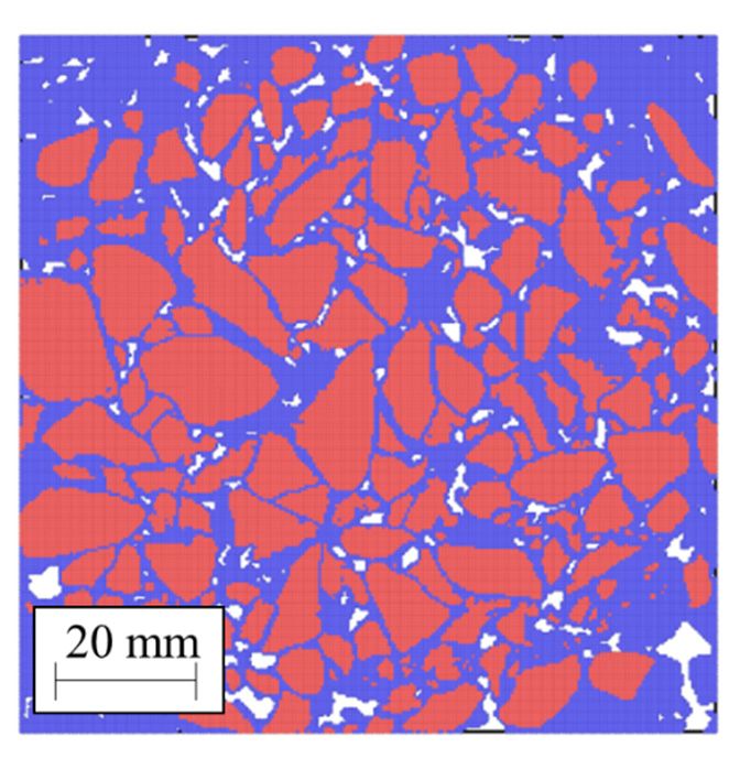
Materials 2021, 14, 1579 6 of 19

 The numerical models, after validation, were used to simulate compressive tests on
 asphalt before and after being subjected to a cycle of freeze-thaw. The damage progression
 under compressive loading and the freeze-thaw was evaluated and discussed with the
 aim of the numerical results obtained. The details of the numerical analyses and the input
 parameters used are also presented in this section.

 3.1. Mixtures
 The asphalt models used in the simulations were derived from samples of four types
 of asphalts: Dense Asphalt (DA), Porous Asphalt #1 (PA #1), Porous Asphalt #2 (PA #2)
 and Porous Asphalt #3 (PA #3), with target air voids of 5 10, 13 and 21%, respectively. The
 physical samples were prepared in the NTEC laboratories at the University of Notting-
 ham, Nottingham, UK. CT-scanned and (as explained later) digitalised in a format reada-
 ble by the software used to carry out the simulations.
 The composition, aggregate gradation and binder contents in the samples are shown
 in Table 2. For all mixtures, crushed limestone aggregates with a maximum size of 20 mm
 and 50/70 pen bitumen were used. The standards BS EN 13043:2013 for DA, BS EN 13108-1
 for PA and BS EN 12697–33 were followed to manufacture the materials [44]. The materi-
 als were mixed at 160 °C and roller compacted at 140 °C. Asphalt slabs of 300 × 300 × 50
 mm3 were produced. From the DA slab, a 35 × 35 × 55 mm3 was cut. From the slabs made
 of PA #1, PA #2 and PA #3, cores of 100 mm diameter and 50 mm height were extracted.

 Table 2. Asphalt mixture composition.

 Size (mm) Passing (%) DA Passing (%) PA #1 Passing (%) PA #2 Passing (%) PA #3
 20 0.9 0.0 20 10
 14 15.8 0.0 25 38
 10 21.3 35.1 26 35
 6.3 14.2 19.3 7 0
 Dust 47.8 45.6 22 17
 Bitumen 4.7 4.5 4.2 3.3
 Air void content 5.0 10.0 13 21

 3.2. DA Model
 The DA sample surface was photographed using a digital camera with resolution
 1257 × 896 and the pictures converted in a black and white image with MATLAB R2020a
 (The Math Works, Inc., Natick, MA, USA) and over imposed on a square lattice with side
 l = 10−4 m. Each node of the lattice corresponds to a Peridynamic particle: blue particles
 were created to represent mastic and red particles to represent aggregates, see Figure 3.
 According to the reference [45], aggregates greater than 1.18 mm can be considered part
 of the solid skeleton structure. Hence, mastic was defined as a mixture of aggregates ≤
 1.18 mm and bitumen. While we are aware that this is a simplification, we will assume
 that this value remains constant for the mixtures that we studied.
 In DA, voids were not considered due to the difficulty of identifying them using dig-
 ital photography. DA has 190,000 particles for the mastic and 300,000 for the aggregates.

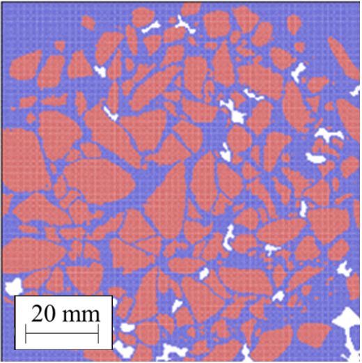
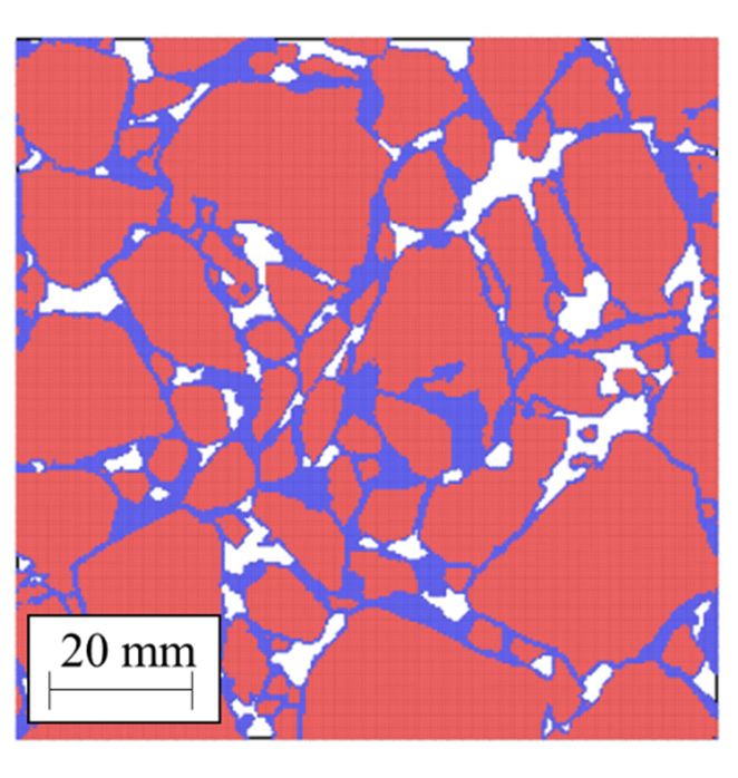
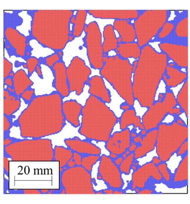
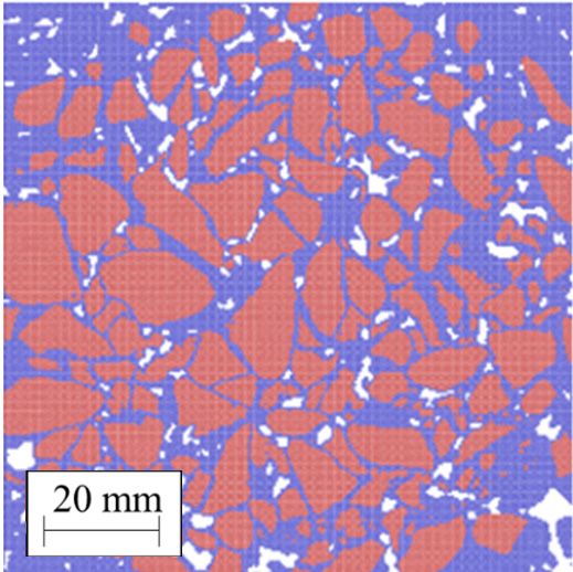
Materials 2021, 14, 1579 7 of 19

 Figure 3. Asphalt (DA): blue particles represent the mortar; red particles represent the aggregate.

 3.3. PA Models
 A Phoenix v|tome|x L 300 micro CT scanner was used to scan PA asphalt samples
 under dry conditions; the X-ray tube was MXR320HP/11 (3.0 mm Be + 2 mm Al) from GE
 Sensing and Inspection Technology (Shanghai, China) operating with an acceleration volt-
 age of 290 kV and a current of 1300 mA.
 We carried out the X-ray CT scans in the micro-computed tomography Hounsfield
 facility at the University of Nottingham, Nottingham, UK. We mounted the samples on a
 rotational table at a distance of 906.84 mm from the X-ray source. The reconstruction of
 scans was performed using GE Datos|x reconstruction software with 2× resolution to ob-
 tain a spatial resolution of 45.2 mm; the scans had an isotropic resolution, meaning that
 the slice thickness was also 45.2 mm. The raw images were 16-bit images, and the voxel
 value represented the x-ray attenuation.
 Then, ImageJ version 1.49 was used to process the images [46], convert them to 8-bit
 grayscale resolution and denoise the images to remove small clusters of voids and grains.
 The different material components such as aggregates, bitumen and air voids were ex-
 tracted by segmenting the images based on grayscale thresholding using ImageJ version
 1.49 (Rasband, W.S., ImageJ, U. S. National Institutes of Health, Bethesda, MD, USA).
 The picture was over imposed on a square lattice with side l = 4 × 10−4 m using Matlab
 2020a. As in the case of DA, each node of the lattice corresponds to a peridynamic particle:
 blue particles are assigned to mastic, and red particles are used to represent aggregates,
 see Figure 3. No computational particle was created in areas corresponding to the voids.
 Since the void fraction and aggregate size differed in the three samples, the number of
 particles was not the same. Sample PA #1 had 341,000 particles for the mortar and 367,000
 for the aggregates; PA #2 148,000 particles for the mortar and 538,500 for the aggregates;
 PA #3 172,000 particles for the mortar and 455,000 particles for the aggregates.

 3.4. Additional Asphalt Geometries
 To generate new geometries of asphalt mixtures with a range of air void properties,
 using ImageJ, we assumed that the mixtures from Figure 4 were the reference. From each
 of these specimens, we produced five different materials. (i) Without air voids; (ii) with
 the 25% smallest air voids; (iii) with the 50% smallest air voids; (iv) with 75% of the small-
 est air voids and (v) with 100% of the air voids (equivalent to the reference sample). See
 an example in Figure 5. The air voids’ geometries, including the average void area, diam-
 eter, perimeter, circularity and aspect ratio, were measured using the Particle Analysis
 function in ImageJ [45]. Finally, a suffix indicating the final void fraction was assigned to
 each generated sample. For example, PA #1/2.5% means that we started from PA #1 and
 filled all the voids so that the final void fraction was 2.5%. The aggregate gradation and
 binder contents are shown in Table 3. Increasing the amount of mastic, we add bitumen
 and dust smaller than 1.18 mm, keeping the skeleton structure constant.

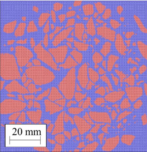
Materials 2021, 14, 1579 8 of 19

 (a) (b) (c)
 Figure 4. Samples (a) PA #1; (b) PA #2; (c) PA #3. Blue particles represent the mortar, red particles the aggregate.

 (a) (b) (c)
 Figure 5. Examples of PA #1 with a range of air void contents. (a) 0%; (b) 5 %; and (c) 10 %.

 Table 3. Asphalt mixture composition.

 Passing (%)
 PA#1 PA#1 PA #1 PA #1 PA#2 PA#2 PA#2 PA #2 PA#3 PA#3 PA#2 PA #3
 Size (mm)
 7.5% 5% 2.5% 0% 9.75% 6.5% 3.25% 0% 15.75% 10.5% 5.25% 0%
 20 0.0 0.0 0.0 0.0 19.5 19.0 18.5 18.1 9.8 9.2 8.9 8.6
 14 0.0 0.0 0.0 0.0 24.5 23.8 23.2 22.7 36.3 35.0 33.5 32.3
 10 34.5 33.9 33.3 32.5 25.3 24.7 24.1 23.5 33.4 32.2 30.9 29.7
 6.3 18.9 18.5 18.2 18.0 6.8 6.7 6.6 6.4 0.0 0.0 0.0 0.0
 Dust above
 30.0 29.4 28.8 28.4 8.8 8.6 8.4 8.3 6.7 6.4 6.2 6.0
1.18 mm [46]
Dust below
 16.6 18.2 19.7 21.1 15.1 17.2 19.2 21.0 13.8 17.2 20.5 23.4
1.18 mm [46]
 Bitumen 5.2 5.9 6.5 7.1 5.2 6.2 7.0 7.9 5.1 6.8 8.2 9.5
 Air void
 7.5 5.0 2.5 0.0 9.75 6.5 3.25 0 15.75 10.5 5.25 0
 content

 Table 4 shows the topological properties of air voids in asphalt mixtures produced in
 this section. Similar results were presented in [12]. These results will be used below to
 evaluate the influence of freezing on the degradation of pavements.

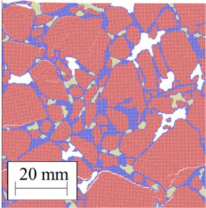
Materials 2021, 14, 1579 9 of 19

 Table 4. Topological properties of the voids calculated from the CT-scans.

 Mean Void Di- Mean Void As- Mean Void Cir-
 Void Content Mean Void Area Mean Void Pe-
 Sample ameter pect Ratio cularity
 [%] [mm2] rimeter [mm]
 [mm] [—] [—]
 PA #1/0% 0.00 0.00 0.00 0.00 0.00 0.00
 PA #1/2.5% 2.50 1.19 1.11 2.80 1.87 0.72
 PA #1/5% 5.00 1.47 1.70 3.63 1.99 0.67
 PA #1/7.5% 7.50 1.67 2.19 4.27 2.03 0.65
 PA #1/10% 10.00 1.82 2.60 4.82 2.03 0.64
 PA #2/0% 0.00 0.00 0.00 0.00 0.00 0.00
 PA #2/3.25% 3.25 2.22 3.87 7.83 2.41 0.54
 PA #2/6.5% 6.50 3.29 8.50 10.05 2.41 0.51
 PA #2/9.75% 9.75 3.82 11.46 11.60 2.38 0.49
 PA #2/13% 13.00 3.42 9.18 13.48 2.40 0.48
 PA #3/0% 0.00 0.00 0.00 0.00 0.00 0.00
 PA #3/5.25% 5.25 3.73 10.92 20.75 2.29 0.48
 PA #3/10.5% 10.50 4.79 18.01 23.80 2.11 0.49
 PA 3/15.75% 15.75 5.57 24.35 23.95 2.16 0.47
 PA #3/21% 21.00 6.06 28.83 19.36 2.11 0.51

 3.5. Freeze-Thaw Simulation
 We only used PA #2, which has a 13% air void content, to evaluate the effect of freeze-
 thaw on mechanical properties. For this purpose, we artificially filled some of the voids
 with ice, presented as yellow particles in Figure 6. To distinguish among samples, a suffix
 indicating the final ice content was assigned to each generated sample. For example, PA
 #2/0.65% means that we started from PA #2 and filled all the voids so that the final ice
 content was 0.65%. Figure 6 shows how this process was carried out. We started with the
 real PA #2 sample whose void fraction was 13%. Then, we gradually covered some of the
 voids (chosen randomly) with ice (yellow particles) until the ice content was 0.65%, Figure
 6a, 1.3%, Figure 6b, 3.25%, Figure 6c, 6.5%, Figure 6d, 9.75%, Figure 6e and finally 13%,
 Figure 6f. The freeze-thaw simulation was performed following these steps:
 • Water expands in the voids simulating ice formation, leading to cracking.
 • After the water expansion is completed, the simulation is carried out for additional
 106 time steps to relax the system with no external load.
 • Water shrinks in the void, simulating ice melting.
 • Water is removed.
 • After the water is removed, the simulation is carried out for additional 106 time steps
 to relax the system with no external load.
 • Finally, the sample is tested under simulated compression to assess mechanical re-
 sponse changes after the sample is subjected to a freeze-thawcycle.

 3.6. Numerical Modelling Details and Input Parameters
 The intrinsic properties of the mastic and aggregate were the same for all simulations.
 In this study, we focused on temperatures below −10 °C and, therefore, we used the Peri-
 dynamic model for brittle materials discussed before. The mechanical properties used in
 the simulations of bitumen and asphalt mixtures are reported in Table 5; they were ob-
 tained from [47] and [48]. The peridynamic parameters of the asphalt binder used for the
 simulations are listed in Table 6.
 The calculation of the temperature profile inside the sample would require a non-
 isothermal model (the reader can refer to [37] for modelling heat transfer and phase tran-
 sition with particle methods). During solidification, water remains at 0 °C because of the
 latent heat. The scenario we have in mind is when the water has permeated into the as-
 phalt and freezes. We assume that the external temperature is sufficiently low; as a first
 approximation, the average temperature of the asphalt sample is close to −10 °C.

Materials 2021, 14, 1579 10 of 19

 To simulate a uniaxial compressive test, each sample is placed into the simulation
 box between two rigid walls (boundary conditions). The simulations are carried out under
 plane stress conditions. For the model, this implies that we take a parallel slice with a
 thickness larger than the horizon and impose the stress along the z direction equal to zero.
 The physical parameters at the interface were set to the physical parameters of the mastic.
 The upper wall moves downward at a controlled velocity, and the lower wall is fixed.
 Uniaxial compression test simulation is carried out along the y-direction at a compression
 rate of 0.001 m/s; (we verified that quasi-static conditions were achieved at 0.001 m/s), the
 other directions were set to be free to expand or shrink. The time step used in all simula-
 tions was 10−8 s.
 The Peridynamic stress was calculated from the total force per volume, acting
 through the first layer of particles in contact with the upper wall. The resultant force was
 obtained by multiplying the particle’s volume and the average force density of the top
 layer. The simulations were carried out with the Peridynamics package [49] in
 LAMMPS/stable_7Aug2019-foss-2019a (http://lammps.sandia.gov) [50].

 Figure 6. (a) PA #2/0.65% ice; (b) PA #2/1.3% ice; (c) PA #2/3.25% ice; (d) PA #2/6.5% ice; (e) PA #2/9.75% ice; (f) PA #2/13%
 ice Ice is represented by yellow particles.

 Table 5. Mechanical properties of bitumen, mastic and aggregates at −10 °C used in the simula-
 tions.

 Material ρ [kg m3] E [GPa] ν [-] G0 [kJ/m2]
 Bitumen, PG64-22 at −18 ℃ [45] 1000 3.7 0.30 —
 Mastic [48] 2200 18.2 0.25 270.00
 Aggregates [48] 2500 56.8 0.15 0.25
 Interface mastic/aggregates [48] — 18.2 0.25 77.00

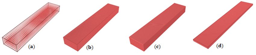
Materials 2021, 14, 1579 11 of 19

 Table 6. Peridynamic parameters used in the simulations. s00 is defined by Equation (9).

 Model l [m] s00 [—] α [—] N
 1 × 10−3 1.2 × 10−4 0.30 3366
 5 × 10−4 1.2 × 10−4 0.30 23,331
 Bitumen beams (3D)
 2 × 10−4 1.2 × 10−4 0.30 332,826
 1 × 10−4 1.2 × 10−4 0.30 2,580,651
 1 × 10−3 2.0 × 10−4 0.30 3927
 5 × 10−4 2.0 × 10−4 0.30 14,847
 Bitumen beams (Thin plate)
 2 × 10−4 2.0 × 10−4 0.30 76,806
 1 × 10−4 2.0 × 10−4 0.30 303,606
 Mastic, DA 1 × 10−4 6.4 × 10−3 0.25 —
 Aggregate, DA 1 × 10−4 1.3 × 10−4 0.25 —
 Interface, DA 1 × 10−4 3.4 × 10−3 0.25 —
 Mastic, PA 4 × 10−4 3.2 × 10−3 0.25 —
 Aggregate, PA 4 × 10−4 6.5 × 10−5 0.25 —
 Interface, PA 4 × 10−4 1.7 × 10−3 0.25 —

 4. Model Validation
 We modelled the tensile strength of bitumen beams tested in [45] to validate the ac-
 curacy of the modelling strategy and its parameters. For this purpose, we produced 3D
 and thin plate (i.e., pseudo 2D with the thickness slightly larger than the horizon simu-
 lated under the plane stress condition) models of the bitumen with different resolutions
 (number of particles used for development of the model) and checked the sensitivity of
 the results to these parameters.
 The 3D specimen had dimensions of 1.0 × 5.0 × 0.5 cm3 simulated with four lattice
 resolutions in the range l = 10−3 – 10−4 m; see Figure 7a–c. In addition, the thin plate speci-
 men had dimensions of 1.0 × 5.0 cm2 and a resolution of l = 10−3 – 10−4 m, see Figure 7d.

 Figure 7. Geometries of bitumen for tensile tests. (a) 3D, l = 10−3 m; (b) 3D, l = 5 × 10−4 m; (c) 3D, l =
 2 × 10−4 m; (d) example of a thin plate, l = 2 × 10−4 m.

 The number of particles in the 3D samples was 3366, 23,331, 332,826 and 2,580,641,
 for l 10−3, 5 × 10−4, 2 × 10−4 and 10−4 m, respectively. The number of particles in the thin
 plates was 3927, 14,847, 76,806 and 303,606, for l 10−3, 5 × 10−4, 2 × 10−4 and 10−4 m, respec-
 tively. The simulations were conducted at the two strain rates, 30 and 140 mm × min−1.
 The Peridynamic stress was calculated from the total force per volume, acting through the
 first layer of particles in contact with the upper wall.
 Figure 8 shows the bitumen’s beam’s failure in a 3D simulation showing that break-
 age is visually comparable with an equivalent experiment from the literature [45].

Materials 2021, 14, 1579 12 of 19

 Figure 8. Broken bitumen sample in the simulation.

 Figure 9a shows the tensile results of the 3D beam. Results are independent of the
 loading rate, and when the particle resolution is l < 2 × 10−4 m, simulations are very close
 to the experimental data. Figure 9b shows the 2D (thin plate) results. For l < 2 × 10−4 m, the
 results are independent of the particle resolution. However, contrary to the 3D results,
 they do not converge to the experimental data. In 2D, the greatest difference between the
 experiment and simulation is 10%. However, the 3D simulation at l = 10−4 m has eight
 times as many particles as the 2D simulation at the same resolution, which makes the
 simulation 16 times slower. Therefore, we decided to accept the error and run the simula-
 tions for thin plates at lattice l = 10−4 m.

 (a) (b)
 Figure 9. Stress/strain of bitumen beams at different resolutions and loading rate and comparison with other experiments
 [45]. (a) In 3D and (b) as a thin plate.

 5. Results and Discussion
 5.1. Compressive Response of DA Asphalt
 The result for the uniaxial compression test for each sample is shown Figure 10a. The
 stress-strain curve follows an equivalent tendency to that of experimental curves reported
 in the literature for asphalt at low temperatures showing brittle behaviour [51]. As ex-
 pected, the stress increases with the compression, undergoing a sudden fracture and lead-
 ing to total failure of the samples.
 The stress-strain curve and the percentage of broken Peridynamic bonds (damage) in
 the sample are compared in Figure 10a to illustrate the relationship between stress and
 damage. Two stages from the stress-strain curve can be distinguished during the failure
 process [52]. In Stage I (strain < 0.015%), there are no obvious cracks. Stage II occurs when
 the local strain reaches the critical value s0. Some of the bonds begin to break, generating
 micro-cracks in the aggregate. As the strain increases further, micro-cracks propagate,
 weakening the material, and the load exceeds the ultimate strength of the sample; micro-

Materials 2021, 14, 1579 13 of 19

 cracks evolve around the aggregates, resulting in large deformations and ultimately the
 destruction of the sample. Finally, Figure 10b shows that micro-cracks form mainly in the
 aggregate, especially at the interfaces, which can be considered the asphalt’s weak part.

 (a) (b)
 Figure 10. (a) Stress (blue curve) and the fraction of broken bond (damage, orange curve) versus strain. (b) Micro-crack
 formation in an asphalt specimen.

 5.2. Compressive Response of PA Asphalt
 Uniaxial compression tests of the PA test specimens mentioned above were also sim-
 ulated to determine whether the peridynamics could capture the air voids’ influence on
 the asphalt’s compression strength. All the samples were subjected to the same load and
 boundary conditions as the DA samples. Figure 10 compares stress/strain curves for PA
 #1, PA #2 and PA #3, in the range of the air void contents studied.
 According to Figure 11, the asphalt stiffness and the peak load decrease by increasing
 the number of voids and their size. The maximal stress decreased by 64% (PA #1), 77%
 (PA #2) and 91% (PA #3) compared to the same asphalt with no voids, and the weakening
 of the material led to early breakage. In real asphalt, this could mean that the weakening
 of the material due to air voids’ presence leads to early breakage [2,30]. Hence, to produce
 durable asphalt, especially at lower temperatures, when the asphalt is prone to ravelling,
 it is advised that the content of mastic in the material is maximised.

 Figure 11. Stress/strain curves for PA #1 (a), PA #2 (b) and PA #3 (c) samples.

Materials 2021, 14, 1579 14 of 19

 There are different types of asphalts that cover a wide range of compressive strengths
 depending on the bitumen, aggregate, fillers and voids. Our asphalt is in line with the
 compressive results for asphalts reported in the literature e.g. [53–55] at the same temper-
 ature. According to the sample and the void fraction, the model’s values in Figure 10 are
 between 0.5 and 3.5 MPa. Reference [53] reports values between 1.5 and 1.9 MPa, reference
 [54] between 2 and 3 MPa and [55] between 1.7 and 2.2 MPa, which are in the same range
 as our simulations. The model’s compressive results depend on the choice of parameters,
 and specifically G0, the fracture energy reported in Table 5, used in the simulations. G0
 was taken from [48] and refers to weakly aggregated dolomite limestone [48], normally
 used to build road bases or binder courses. Hence, the compressive strength of asphalt
 will reflect the poor properties of these aggregates. Properties of additional aggregates
 can be found in reference [56].
 Table 7 reports the Pearson’s correlation between the mechanical and the topological
 properties of the samples. The max stress and the max deformations are, respectively, the
 maximal stress and deformation before the sample’s failure, while for the equivalent
 Young’s Modulus, the slope of the linear part of the stress/strain curve, see Figure 11.
 As expected, a higher void content reduces the uniaxial compressive strength of the
 asphalt. Table 7 also shows that larger voids are more detrimental than smaller voids for
 the same void content. Moreover, given the same void size, samples with elongated and
 irregular shapes (i.e., high aspect ratio, low circularity) show, in general, lower ultimate
 strength and an equivalent Young’s modulus than samples with circular-like voids. The
 reasons for this are still unclear and will be investigated in future research.

 Table 7. Pearson correlations between the mechanical and the topological properties of the samples.

 Mean Void Diameter Mean Void Aspect Mean Void Circu-
 Properties Void Content Mean Void Area
 [mm] Ratio larity
 Ultimate strength −0.62 −0.64 −0.58 −0.52 −0.37
 Ultimate strain −0.77 −0.92 −0.82 −0.73 −0.41
Equivalent Young modulus −0.26 0.02 0.09 −0.32 −0.57
 To compare changes of strength between the different types of asphalt analysed due
 to changes in gradation and amount of mastic, we have defined the parameter β as:
 maximal strength of the asphalt sample
 = 1− × 100 (21)
 maximal strength of asphalt with 0% air voids
 Finally, Figure 12 shows how β varies with the air voids fraction for PA #1, PA #2 and
 PA #3. It can be observed that small changes in the void fraction have a lower influence
 on the compressive strength of asphalt for densely packed mixtures. However, other types
 of mixtures, such as PA #3, could be extremely sensitive to changes in the amount of voids,
 for example, due to the lack of filler or changes in the source of dust, and extreme care
 should be taken during their design and manufacturing. This will be a point that we will
 analyse experimentally in future research.

Materials 2021, 14, 1579 15 of 19

 Figure 12. Changes of with void %.

 5.3. Effect of Freeze-thawon the Compressive Strength
 Figure 13 shows the sample during the ice expansions. Breakage starts where ice ex-
 pands and propagates at the bitumen-aggregate interface. This also creates new voids and
 increases the void fraction [7]. As expected, the freeze-thawcycle decreases the strength of
 asphalt [57–59]. To quantify this decrease and compare the simulations with experimental
 data, we define the reduction of the peak stress after freeze-thawas follows:
 peak stress of the sample after freeze − thaw
 γ= 1− × 100 (22)
 peak stress of the intact sample

 (a) (b)
 Figure 13. Cracking propagation due to ice expansion: (a) geometry; (b) damage.

 Figure 14 shows how γ varies with the ice fraction and confirms the ice’s impact on
 fracture performance. During the ice expansion, cracks appear in the structure, and the
 stiffness of asphalt is compromised, leading to a reduction in the sample’s peak stress and
 earlier failure.

Materials 2021, 14, 1579 16 of 19

 Figure 14. Reduction of peak stress with ice %.

 These results compare with experimental data. For example, reference [9] has deter-
 mined that for a porous asphalt mixture with approximately 20% air void content, the
 strength loss can be higher than 40%. Further, most of the strength is lost after the first
 cycle, as shown in Figure 13. In future research, this computational framework will be
 used to better understand the influence of air voids’ geometrical properties on the re-
 sistance of the asphalt to freeze-thawcycles.

 6. Conclusions
 In this article, we have demonstrated the use of Peridynamics combined with Dis-
 crete Multiphysics to model crack formation and propagation in asphalt at low tempera-
 tures taking into account air voids and ice formation. Find below some of the conclusions:
 • This paper demonstrates a way to understand how microcracks are formed in the
 asphalt under freezing conditions, a phenomenon that is extremely difficult to ob-
 serve in experiments.
 • The simulations show the model’s reliability in obtaining a mechanical response
 comparable with experimental tension and compression tests of bitumen and as-
 phalt, respectively.
 • As expected, the higher the void fraction, the higher the loss of compressive strength
 of an asphalt mixture. Further, the size and shape of the voids affect the strength of
 the asphalt. Larger voids are more detrimental than smaller voids, especially if they
 have a high aspect ratio and low circularity.
 • Using this model, we observed that the amount of mastic in densely packed mixtures
 does not have a strong influence on the compressive strength of asphalt. However,
 less densely packed mixtures, such as porous asphalt, are more sensitive to the
 amount of mastic in the asphalt.
 • The model can also assess the effect of ice formation on the asphalt structure. Water
 particles are created in the voids, and their volume is increased with time to simulate
 solidification. The simulations show the formation of cracks produced by water ex-
 pansion during solidification and the consequent loss in mechanical strength. To the
 best of our knowledge, water expansion in cavities has not been simulated to date.
 This methodological study provides researchers in the field with a powerful new tool
 for understanding the behaviour of asphalt under scenarios that, so far, have not been
 accessible to computer simulation. The systematic study of asphalt mechanical properties
 changes due to the size, number and distribution of ice-filled voids will be done in future
 research.

Materials 2021, 14, 1579 17 of 19

 Author Contributions: Conceptualisation, D.S., B.G., A.A., A.G.H.; methodology, All authors; soft-
 ware, D.S, B.G., A.A.; validation, D.S.; formal analysis, D.S.; investigation, D.S.; resources, All au-
 thors; data curation, D.S.; writing—original draft preparation, All authors; writing—review and ed-
 iting, All authors; visualisation, All authors; supervision, B.G. A.A., A.G.H. All authors have read
 and agreed to the published version of the manuscript.
 Funding: PhD fund lead to this study was provided by the Faculty of Engineering of the University
 of Notitngham and the School of Chemical Engineering of the University of Birmingham.
 Institutional Review Board Statement: Not applicable.
 Informed Consent Statement: Not applicable.
 Data Availability Statement: The code used for the simulations is freely available under the GNU
 General Public License v3 and can be downloaded from the University of Birmingham repository
 http://edata.bham.ac.uk/568/.
 Acknowledgments: The authors express their gratitude to the Universities of Nottingham, Birming-
 ham and Highways England UK that funded this study.
 Conflicts of Interest: The authors declare no conflict of interest.

References
1. Bobiński, J.; Tejchman, J. A coupled constitutive model for fracture in plain concrete based on continuum theory with non-local
 softening and eXtended Finite Element Method. Finite Elements Anal. Des. 2016, 114, 1–21.
2. Suchorzewski, J.; Tejchman, J.; Nitka, M. Discrete element method simulations of fracture in concrete under uniaxial compres-
 sion based on its real internal structure. Int. J. Damage Mech. 2018, 27, 578–607.
3. Ling, M.; Zhang, Y.; Kaseer, F.; Martin, A.E.; Lytton, R.L. Investigation of fracture behavior of asphalt mixture composite using
 energy-based approach. Compos. Part B Eng. 2020, 181, 107324.
4. Kollmann, J.; Liu, P.; Lu, G.; Wang, D.; Oeser, M.; Leischner, S. Investigation of the microstructural fracture behaviour of asphalt
 mixtures using the finite element method. Constr. Build. Mater. 2019, 227, 117078.
5. Ozgan, E.; Serin, S. Investigation of certain engineering characteristics of asphalt concrete exposed to freeze-thawcycles. Cold
 Reg. Sci. Technol. 2013, 85, 131–136.
6. Tang, N.; Sun, C.; Huang, S.; Wu, S. Damage and corrosion of conductive asphalt concrete subjected to freeze-thawcycles and
 salt. Mater. Res. Innov. 2013, 17, 240–245.
7. Xu, H.; Guo, W.; Tan, Y. Internal structure evolution of asphalt mixtures during freeze-thawcycles. Mater. Des. 2015, 86, 436–
 446, doi:10.1016/j.matdes.2015.07.073.
8. Butkovich, T.R. Thermal Expansion of Ice. J. Appl. Phys. 1959, 30, 350, doi:10.1063/1.1735166.
9. Sol-Sánchez, M.; Moreno-Navarro, F.; García-Travé, G.; Rubio-Gámez, M.C. Laboratory study of the long-term climatic deteri-
 oration of asphalt mixtures. Constr. Build. Mater. 2015, 88, 32–40, doi:10.1016/j.conbuildmat.2015.03.090.
10. Xu, H.; Guo, W.; Tan, Y. Permeability of asphalt mixtures exposed to freeze-thawcycles. Cold Reg. Sci. Technol. 2016, 123, 99–106,
 doi:10.1016/j.conbuildmat.2020.118043.
11. Aboufoul, M.; Shokri, N.; Saleh, E.; Tuck, C.; Garcia, A. Dynamics of water evaporation from porous asphalt. Constr. Build.
 Mater. 2019, 202, 406–414, doi:10.1016/j.conbuildmat.2019.01.043.
12. Aboufoul, M.; Garcia, A. Factors affecting hydraulic conductivity of asphalt mixture. Mater. Struct. Mater. Constr. 2017, 50, 116,
 doi:10.1617/s11527-016-0982-6.
13. Hernandez-Fernandez, N.; Underwood, B.S.; Ossa-Lopez, A. Simulation of the asphalt concrete stiffness degradation using
 simplified viscoelastic continuum damage model. Int. J. Fatigue 2020, 140, 105850, doi:10.1016/j.ijfatigue.2020.105850.
14. Li, Y.; Jiang, W.; Shan, J.; Li, P.; Lu, R.; Lou, B. Characteristics of void distribution and aggregate degradation of asphalt mixture
 specimens compacted using field and laboratory methods. Constr. Build. Mater. 2020, 270, 121488,
 doi:10.1016/j.conbuildmat.2020.121488.
15. Canestrari, F.; Ingrassia, L.P. A review of top-down cracking in asphalt pavements: Causes, models, experimental tools and
 future challenges. J. Traffic Transp. Eng. Engl. Ed. 2020, 7, 541–572, doi:10.1016/j.jtte.2020.08.002.
16. Liu, H.; Zeiada, W.; Al-Khateeb, G.G.; Shanableh, A.; Samarai, M. Use of the multiple stress creep recovery (MSCR) test to
 characterize the rutting potential of asphalt binders: A literature review. Constr. Build. Mater. 2020, 269, 121320,
 doi:10.1016/j.conbuildmat.2020.121320.
17. Yan, K.; Ge, D.; You, L.; Wang, X. Laboratory investigation of the characteristics of SMA mixtures under freeze-thawcycles. Cold
 Reg. Sci. Technol. 2015, 119, 68–74.
18. Fan, Z.; Xu, H.; Xiao, J.; Tan, Y. Effects of freeze-thawcycles on fatigue performance of asphalt mixture and development of
 fatigue-freeze-thaw(FFT) uniform equation. Constr. Build. Mater. 2020, 242, 118043.
19. Cong, L.; Ren, M.; Shi, J.; Yang, F.; Guo, G. Experimental investigation on performance deterioration of asphalt mixture under
 freeze-thawcycles. Int. J. Transp. Sci. Technol. 2020, 9, 218–228, doi:10.1016/j.ijtst.2020.04.004.

Materials 2021, 14, 1579 18 of 19

20. Zhang, Z.N.; Chen, Y.X. Modeling nonlinear elastic solid with correlated lattice bond cell for dynamic fracture simulation.
 Comput. Methods Appl. Mech. Eng. 2014, 279, 325–347.
21. Zhao, G.F.; Fang, J.N.; Zhao, J. A 3D distinct lattice spring model for elasticity and dynamic failure. Int. J. Numer. Anal. Methods
 Geomech. 2011, 35, 859–885.
22. Jiang, C.; Zhao, G.F.; Khalili, N. On crack propagation in brittle material using the distinct lattice spring model. Int. J. Solids
 Struct. 2017, 118-119, 41–57, doi:10.1016/j.ijsolstr.2017.04.024.
23. Silling, S.A. Reformulation of elasticity theory for discontinuities and long-range forces. J. Mech. Phys. Solids 2000, 48, 175–209,
 doi:10.1016/s0022-5096(99)00029-0.
24. Pazdniakou, A.; Adler, P.M. Lattice Spring Models. Transp. Porous Media 2012, 93, 243–262, doi:10.1007/s11242-012-9955-6.
25. Mitchell, J.A. A Nonlocal, Ordinary, State-Based Plasticity Model for Peridynamics. Sandia Report, May, 1–34. Available online:
 http://www.ntis.gov/help/ordermethods.asp?loc=7-4-0#online (29 May 2020).
26. Mitchell, J.A. Non-Local, Ordinary-State-Based Viscoelasticity Model for Peridynamics; Sandia Report, SAND2011-8(October); Sandia
 National Laboratories: Albuquerque, NM, USA, 2011; 28p.
27. Alexiadis, A. The Discrete Multi-Hybrid System for the simulation of solid-liquid flows. PLoS ONE 2015, 10, e0124678.
28. Alexiadis, A. A smoothed particle hydrodynamics and coarse-grained molecular dynamics hybrid technique for modelling
 elastic particles and breakable capsules under various flow conditions. Int. J. Numer. Methods Eng. 2014, 100, 713–719.
29. Alexiadis, A. A new framework for modelling the dynamics and the breakage of capsules, vesicles and cells in fluid flow.
 Procedia UTAM 2015, 16, 80–88.
30. Silling, S.A.; Askari, E. A meshfree method based on the peridynamic model of solid mechanics. Comput. Struct. 2005, 83, 1526–
 1535, doi:10.1016/j.compstruc.2004.11.026.
31. Silling, S.A.; Epton, M.; Weckner, O.; Xu, J.; Askari, E. Peridynamic States and Constitutive Modeling. J. Elast. 2007, 88, 151–184,
 doi:10.1007/s10659-007-9125-1.
32. Ha, Y.D.; Bobaru, F. Studies of dynamic crack propagation and crack branching with peridynamics. Int. J. Fract. 2010, 162, 229–
 244, doi:10.1007/s10704-010-9442-4.
33. Ariane, M.; Wen, W.; Vigolo, D.; Brill, A.; Nash, G.B.; Barigou, M.; Alexiadis, A. Modelling and simulation of flow and agglom-
 eration in deep veins valves using Discrete Multi Physics. Comput. Biol. Med. 2017, 89, 96–103.
34. Ariane, M.; Kassinos, S.; Velaga, S.; Alexiadis, A. Discrete multi-physics simulations of diffusive and convective mass transfer
 in boundary layers containing motile cilia in lungs. Comput. Biol. Med. 2018, 95, 34–42.
35. Schütt, M.; Stamatopoulos, K.; Batchelor, H.K.; Simmons, M.J.H.; Alexiadis, A. Modelling and simulation of the hydrodynamics
 and mixing profiles in the human proximal colon using. Discret. Multiphys. Comput. Biol. Med. 2020, 121, 103819.
36. Rahmat, A.; Barigou, M.; Alexiadis, A. Numerical simulation of dissolution of solid particles in fluid flow using the SPH method.
 Int. J. Numer. Methods Heath Fluid Flow 2019, 30, 290–307.
37. Alexiadis, A.; Ghraybeh, S.; Geng, Q. Natural convection and solidification of phase-change materials in circular pipes: A SPH
 approach. Comput. Mater. Sci. 2018, 150, 475–483.
38. Ariane, M.; Allouche, H.; Bussone, M.; Giacosa, F.; Bernard, F.; Barigou, M.; Alexiadis, A. Discrete multiphysics: A mesh-free
 approach to model biological valves including the formation of solid aggregates at the membrane surface and in the flow. PLoS
 ONE 2017, 12, e0174795.
39. Ariane, M.; Vigolo, D.; Brill, A.; Nash, G.B.; Barigou, M.; Alexiadis, A. Using Discrete Multi-Physics for studying the dynamics
 of emboli in flexible venous valves. Comput. Fluids 2018, 166, 57–63.
40. Rahmat, A.; Barigou, M.; Alexiadis, A. Deformation and rupture of compound cells under shear: A Discrete Multiphysics Study.
 Phys. Fluids 2019, 31, 051903.
41. Alexiadis, A. Deep Multiphysics and Particle–Neuron Duality: A Computational Framework Coupling (Discrete) Multiphysics
 and Deep Learning. J. Appl. Sci. 2019, 9, 5369.
42. Alexiadis, A. Deep Multiphysics: Coupling Discrete Multiphysics with Machine Learning to attain self-learning in-silico models
 replicating human physiology. Artif. Intell. Med. 2019, 98, 27–34.
43. Kot, M.; Nagahashi, H.; Szymczak, P. Elastic moduli of simple mass spring models. Vis. Comput. 2015, 31, 1339–1350,
 doi:10.1007/s00371-014-1015-5.
44. BS EN 12697-33. Bituminous Mixtures, Test Methods for Hot Mix Asphalt: Specimen Prepared by Roller Compactor; BSI: London, UK,
 2003.
45. Guarin, A.; Roque, R.; Kim, S.; Sirin, O. Disruption factor of asphalt mixtures. Int. J. Pavement Eng. 2013, 14, 472–485,
 doi:10.1080/10298436.2012.727992.
46. Ferreira, T.; Rasband, W.S. “ImageJ User Guide—IJ 1.46”, 2010—2012. Available online:
 https://imagej.nih.gov/ij/docs/guide/ (accessed on 16 July 2020)
47. Mirsayar, M.M. On the low temperature mixed mode fracture analysis of asphalt binder—Theories and experiments. Eng. Fract.
 Mech. 2017, 186, 181–194.
48. Kim, H.; Buttlar, W.G. Multi-scale fracture modeling of asphalt composite structures. Compos. Sci. Technol. 2009, 69, 2716–2723,
 doi:10.1016/j.compscitech.2009.08.014.
49. Parks, M.L.; Lehoucq, R.B.; Plimpton, S.J.; Silling, S.A. Implementing peridynamics within a molecular dynamics code. Comput.
 Phys. Commun. 2008, 179, 777–783.
50. Plimpton, S. Fast Parallel Algorithms for Short-Range Molecular Dynamics. J. Comput. Phys. 1995, 117, 1–19.

Materials 2021, 14, 1579 19 of 19

51. Kong, X.M.; Liu, Y.L.; Zhang, Y.R.; Zhang, Z.L.; Yan, P.Y.; Bai, Y. Influences of temperature on mechanical properties of cement
 asphalt mortars. Mater. Struct. 2014, 47, 285–292, doi:10.1617/s11527-013-0060-2.
52. Li, W.; Guo, L. Meso-fracture simulation of cracking process in concrete incorporating three-phase characteristics by peri-
 dynamic method. Constr. Build. Mater. 2018, 161, 665–675, doi:10.1016/j.conbuildmat.2017.12.002.
53. Cheng, Y.; Li, H.; Wang, W.; Li, L.; Wang, H. Laboratory evaluation on the performance degradation of styrene-butadiene-
 styrene-modified asphalt mixture reinforced with basalt fiber under freeze-thawcycles. Polymers 2020, 12, 1092,
 doi:10.3390/polym12051092.
54. Wang, F.; Liu, Z.; Wang, T.; Hu, S. Temperature stability of compressive strength of cement asphalt mortar. ACI Mater. J. 2010,
 107, 27–30, doi:10.14359/51663461.
55. Si, W.; Ma, B.; Wang, H.; Hu, J. Analysis on splitting characteristics of asphalt mixture under freeze-thawcycles in cold plateau
 regions. Transp. Sci. Eng. 2013, 37, 805–808, doi:10.3963/j.issn.2095-3844.2013.04.032.
56. Li, X.; Braham, A.F.; Marasteanu, M.O.; Buttlar, W.G.; Williams, R.C. Effect of factors affecting fracture energy of asphalt con-
 crete at low temperature. Road Mater. Pavement Des. 2008, 9, 397–416, doi:10.3166/RMPD.9HS.397-416.
57. Din, I.M.U.; Mir, M.S.; Farooq, M.A. Effect of Freeze-thawCycles on the Properties of Asphalt Pavements in Cold Regions: A
 Review. Transp. Res. Procedia 2020, 48, 3634–3641, doi:10.1016/j.trpro.2020.08.087.
58. Meng, Y.; Li, Z.-Y.; Mei, Y.-J.; Lu, Y.-F. Temperature Modification Coefficient of compressive modulus of asphalt mixture. J.
 Tongji Univ. Nat. Sci. Ed. 2008, 2, 182–186.
59. Tan, Y.; Zhao, L.; Lan, B.; Meng, L. Research on Freeze-thawDamage Model and Life Prediction of Asphalt Mixture. J. Highw.
 Transp. Res. Dev. 2011, 6, 1–7.