Knud Rasmussen Glacier Status Analysis Based on Historical Data and Moving Detection Using RPAS - Preprints.org
←
→
Page content transcription
If your browser does not render page correctly, please read the page content below
Preprints (www.preprints.org) | NOT PEER-REVIEWED | Posted: 1 December 2020                          doi:10.20944/preprints202012.0006.v1

                  Article
                  Knud Rasmussen Glacier Status Analysis Based on
                  Historical Data and Moving Detection Using RPAS
                  Karel Pavelka 1        , Jaroslav Šedina 1, Karel Pavelka jr.
                    1 Czech Technical University in Prague, Faculty of Civil Engineering, Thakurova 7, Czech Republic;
                      pavelka@fsv.cvut.cz, Jaroslav.sedina@gmail.com, karel.pavelka@hotmail.com
                    * Correspondence: pavelka@fsv.cvut.cz; Tel.: +420-608211360 (KP)

                    Abstract: This article discusses an international scientific expedition to Greenland that researched
                    geography, geodesy, botany, and glaciology of the area. The results here focus on the geodetic and
                    glaciological results obtained with the eBee drone in the eastern part of Greenland at the front of
                    the Knud Rasmussen glacier. From two overflights nearby the glacier front, it was possible to
                    obtain the speed of the glacier flow and the distribution of velocities in the glacier stream. The
                    results correlate with other measurement methods and this technology has been shown as feasible.
                    Of course, there are more accurate and long-term options or devices for monitoring the flow of
                    glaciers. In this case of short-term visits to the site, the possibility of using a drone is interesting and
                    the results show not only the flow speed of the glacier, but also the shape and structure from a
                    height of up to 200m. The second part of the paper focuses on the analysis of modern satellite
                    images of the Knud Rasmussen glacier from Google Earth (Landsat series 1984-2016) and a
                    comparison with historical aerial images from 1932-1933. Experimentally, historical images were
                    processed photogrammetrically into a 3D model.

                    Keywords: Greenland; photogrammetry; Knud Rasmussen Glacier; RPAS;

                  1. Introduction

                  1.1. Dedication
                       I would like to dedicate this article in memoriam to my friend, scientist, and real man, Professor
                  Wilfried Korth (Fig.1.), who tragically died in the spring 2019, just before his last planned expedition
                  to Greenland (KP).

                                                     Figure 1. Professor Wilfried Korth († 2019).

                  1.2. Arctic research
                       Arctic research has been a matter of hundreds of years [1]. Cruises to the north are dated to the
                  16th century. In addition to the scientific goals of the expeditions, there were also prestigious
                  expeditions, which aimed to reach the North Pole of our planet.
                       There is still controversy over who stood as a first one at the North Pole; it is generally claimed
                  that Frederick Cook was the first in 1908, but he could not credibly prove his primacy. Furthermore,
                  the North Pole was reached in 1909 by Edwin Peary, accompanied by a servant Matthew Henson

           © 2020 by the author(s). Distributed under a Creative Commons CC BY license.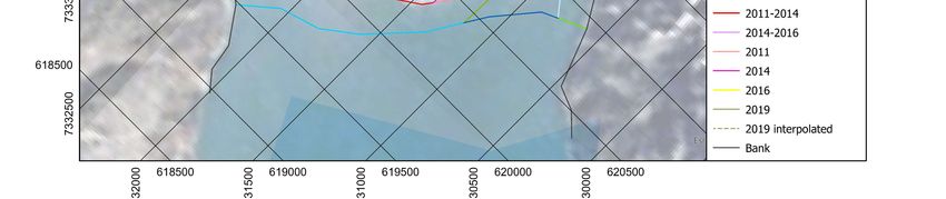
Preprints (www.preprints.org) | NOT PEER-REVIEWED | Posted: 1 December 2020                      doi:10.20944/preprints202012.0006.v1

                  and four Innuits; there is also controversy over his triumph, as well as the first overflight of the
                  North Pole by Richard Byrd and Floyd Bennett in a plane in 1926. The first truly documented
                  achievement of the North Pole was with Norge airship in 1926, onboard with Roald Amundsen,
                  Italian airship designer Umberto Nobile, and Lincoln Ellsworth [2]. In 1928, on the return from the
                  North Pole, the airship Italia with Commander Umberto Nobile crashed. The Czech scientist
                  František Běhounek was also a member of the crew [3], and survived the expedition; part of the team
                  was saved later by the Soviet icebreaker Krasin. Unfortunately, the polar explorer Roald
                  Ammundsen, the pilot and crew died in the rescue operation.
                        This article deals with the research of Greenland. Greenland was discovered after 982 by the
                  Viking Erik the Red. Thanks to the warmer climate, the Vikings lived there until the middle (maybe
                  till the end) of the 14th century, when a global cooling started. Until the 18th century, only Inuit
                  people who migrated from North America lived there, later Europeans and Americans began to
                  infiltrate Greenland and established trade settlements. Since the beginning of the 19th century,
                  Greenland has been a part of Denmark, and since 1979 it has had extensive autonomy with its own
                  parliament. Due to the gradual warming and melting of the Greenland Glacier, Greenland has great
                  potential for the future thanks to its large reserves of mineral wealth. However, the melting of the
                  Greenland Glacier can have fatal consequences for the whole world [4] .
                        Since the 1980s, ice has been declining more than it is recreated in winter. Winters are milder
                  and summers longer and warmer. The ice that disappears will not be restored. Nowadays, six times
                  more ice has been disappearing from Greenland than in the 1980s [5].
                        The Greenland Glacier is a vast mass of ice covering 1.7 million square kilometres, which
                  represents about 80% of Greenland's surface. It is the second largest glaciated area in the world, first
                  is the Antarctic glacier. Its thickness is usually more than 2 kilometres and sometimes exceeds 3
                  kilometres [6] . The weight of the glacier has compressed the central part of Greenland, bringing the
                  rocky bedrock below it to about sea level, while the mountain range surrounds the glacier almost
                  along its entire edge. This is detectable by the deformation of the Earth's gravity field. If the entire
                  Greenland Glacier melted, the level of the world's oceans would rise by about 7 meters. Due to the
                  long-term melting of the glacier, the compressed rock is gradually rising on the outskirts of
                  Greenland. According to the scientific studies, the Greenland coast rises by 2.5 cm per year [7,8].
                  However, it is also scientifically confirmed that some parts of the glacier are even increasing . This
                  information indicates that the condition of the Greenland Glacier must continue to be carefully
                  studied. Today, scientific satellites in particular are contributing to this [9] .
                        Greenland's scientific research is linked to the significant deeds of travellers, ethnography and
                  polar explorers.
                        One of the first researchers in Greenland was undoubtedly the legendary Fridtjof Nansen
                  (1861-1930). In 1888, he crossed with the six-member group as the first one Greenland´s glacier in the
                  length of about 650 km. He proved that it is covered with ice from the entire interior of Greenland,
                  and obtained a unique set of meteorological measurements. Due to the extreme weather, they spent
                  the winter with the Inuit and could return home an year later [10].
                        Knud Rasmussen (1879-1933) was one of the first and one of the most important polar
                  researchers and ethnographers in Arctic (Fig.2.). He was born in Jakobshavn (Illulisat) into the
                  family of a Danish missionary. He was engaged in ethnography and used a dog sled to travel around
                  a large part of Greenland. During the first of seven expeditions to the north part of Greenland, he
                  founded, among other things, the Thule trading station [11].
Preprints (www.preprints.org) | NOT PEER-REVIEWED | Posted: 1 December 2020                  doi:10.20944/preprints202012.0006.v1

                                                       Figure 2. Knud Rasmussen.

                       In 1912 Alfred de Quervain undertook an important scientific Swiss Greenland Expedition,
                  during which meteorological and geodetic information was measured. He and his team crossed the
                  Greenland Glacier in a north-westerly direction for almost 700 km [12]. It is interesting, that one
                  member of the team was Roderich Fick, the grandfather of Stephan Orth, the participant in a
                  German expedition to the centenary of the expedition of Alfred de Quervain led by Professor
                  Wilfried Korth in 2012 [13], (Fig.3.).

                                        Figure 3. Map of Greenland and the Knud Rasmussen Glacier.
                       (http://www.getamap.net/maps/greenland_%5B_denmark_%5D/ostgronland/_knud_rasmussen_gla
                                                                   cier/)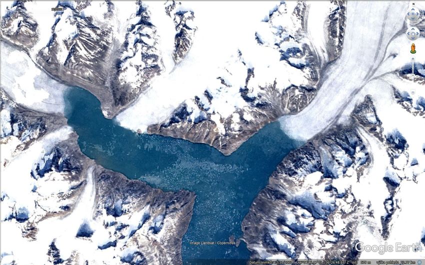
Preprints (www.preprints.org) | NOT PEER-REVIEWED | Posted: 1 December 2020                           doi:10.20944/preprints202012.0006.v1

                       The mapping of Greenland began as early as the 15th century when parts of the coast were
                  mapped. However, systematic mapping was possible only in the 20th century using aerial
                  photogrammetry and later from satellites. A significant achievement was the Danish geodetic
                  expedition in 1931-34. Many aerial photographs were taken using three Heinkel seaplanes. These
                  photographs are perfect source for monitoring the condition of Greenlandic glaciers (Fig.4.).
                       During the seventh Thule Expedition a systematic survey of the southeast coast of Greenland
                  was carried out in 1932–1933. Aerial photographs of the Knud Rasmusen glacier were taken in this
                  time. Nowadays, at the Natural History Museum of Denmark, there is a long-term project called
                  „AirBase “. It is a database which has a quarter millions of aerial photos recorded by Danish survey
                  agencies in the period 1930 to the 1980s. This is a unique source of information about glaciers [14,
                  15].

                         Figure 4. The Knud Rasmussen Glacier in a photo from the Danish Greenland expedition (the
                           seventh Thule Expedition 1932-33); (photo The Arctic Institute, https://arktiskinstitut.dk/).

                  2. University research
                       The Department of Geomatics, Czech Technical University in Prague, Faculty of Civil
                  Engineering, has focused on the documentation of historical monuments and landscape using
                  photogrammetry for a long time, more recently also using laser scanning and geophysical methods
                  [16,17].
                       In 2014, cooperation was established between the Beuth Hochschule für Technik Berlin, TU
                  Cottbus, and the Czech Technical University in Prague, Faculty of Civil Engineering. This was based
                  on contacts between a prominent German polar explorer and surveyor, Professor W. Korth, and
                  Professor K. Pavelka, a specialist in remote sensing and photogrammetry.
                       After consultations and training in Norway, a joint expedition to Greenland was organized in
                  2015. A German group led by Professor W. Korth made research in Greenland since 2002 and
                  crossed the 700 km long Greenland Glacier using skis five times in the footsteps of the Swiss polar
                  explorer Alfred de Quervain. The aim was to measure the profile of the glacier using GNSS
                  equipment and complementary meteorological and glaciological information.
                       The expedition in 2015 consisted of two teams. The first expeditionary team went from the east
                  coast through Greenland to the west, a small support team met the first one at a place called Swiss
                  Camp, about 100km from the west coast on a glacier. Both groups then went further to the ice
                  border, where further experiments were performed. It involved the placement of four radar
                  reflectors to monitor the movement of the glacier using the Terra SAR X satellite, as well as the
                  detection of the movement of the Egi Glacier in Disko Bay using a winged drone. These researches
                  were designed and performed by professor Pavelka from CTU FCE, Prague. The results were
                  applicable and published [18]. The use of a drone proved to be possible and suitable despite the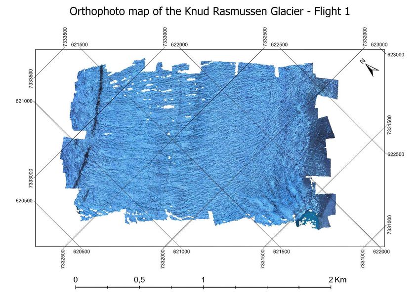
Preprints (www.preprints.org) | NOT PEER-REVIEWED | Posted: 1 December 2020                              doi:10.20944/preprints202012.0006.v1

                  extreme conditions, the impossibility of supporting measurements of control points, and difficult
                  and inaccessible terrain.
                       Following the success of the 2015 expedition, a new expedition with a similar composition was
                  planned for 2019. Sailing with a research ship along the east coast of Greenland was planned and a
                  new crossing over the Greenland Glacier in the same route as during the previous expeditions. By
                  repeating the crossings along the same route and measuring, interesting information should have
                  been obtained about the decrease in ice and climate change.
                       In spring 2019, unfortunately, Professor W. Korth died tragically. After discussions, the
                  already prepared expedition took place, but with a minimal team and without crossing the
                  Greenland Glacier. All that remained was a research ship sailing around a part of the east coast to
                  the famous glaciers near the Kulusuk village and a shorter research voyage to the glacier.

                  2.1. Cruise and planned research
                       The research ship voyage was arranged for me without much information as only Professor W.
                  Korth had the details. After arriving in Kulusuk from Reykjavik (Island), it was necessary to wait for
                  the ship. The situation became complicated because of the weather, the plane did not fly, and I
                  (KP) remained alone from the three-member team on the island with minimal equipment, but with a
                  computer and a disassembled drone. It was necessary to spend some nights with the locals who
                  helped me. Third day, the expedition sailing vessel Dagmar Aaen arrived with the crew and captain
                  Arved Fuchs, a world-famous traveller and researcher. It was a surprise for me, I had no information
                  about it, only an email communication, and a link to Wilfried Korth. Dagmar Aaen is formerly a
                  fishing cutter built in 1931 and adapted by Arved Fuchs to a research expedition ship, which has
                  already made several research voyages to the Arctic. After a short voyage, we picked up a late
                  participant in the expedition, a student Luisa Näke, who participated in the expedition within the
                  Erasmus program and for the future final bachelor's thesis [19], (Fig.5).

                       Figure 5. A research ship sailed around a part of the east coast to the famous glaciers (one week); this
                                                    image was taken in in the navigation cabin.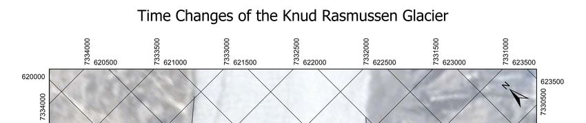
Preprints (www.preprints.org) | NOT PEER-REVIEWED | Posted: 1 December 2020                            doi:10.20944/preprints202012.0006.v1

                       Figure 6. Knud Rasmussen Glacier; it seems to be a small glacier, but its width is over 2km.

                  2.2. Planned research
                       The goal was to select sites within a few days of sailing from Kulusuk, such as researching an
                  abandoned US military base from World War II Bluei East II. and research and measurement of the
                  melting glaciers (Fig.6.). This research is a follow-up to a number of projects focused on the
                  documentation of glaciers using drones and the detection of changes using point clouds [20, 21, 22].

                       The crew consisted of a professionally diverse team from the fields of biology,
                  photogrammetry, reporters, students, and others.
                       Aim of the photogrammetry was to create detailed maps of Bluei East II. and drone research on
                  the movement of glaciers. As the satellite images are out of date or unactual, it was not possible to
                  precisely define the exact parameters and destination of the drone flight. As in 2015, this proved to
                  be a problem. The front of the glacier was hundreds of meters away from the latest satellite images,
                  so the flight plan had to be estimated (Fig. 7-8.).

                  2.3. Flights
                       RPAS (remotely piloted aircraft system) is a less used but correct acronym for a drone. It means
                  that there is a pilot who remotely controls the device - and is therefore responsible for it. The eBee
                  drone was used in this case for different reasons. 1) it is light, made from styrofoam, easy to use,
                  takes off from the hand and lands without a special place, 2) it is easy to transport (in a padded
                  backpack), it can be divided into several parts for transport, electrical powered, using small
                  batteries, 3) it has a relatively long time of flight and altitude access (it is winged drone), 4) it flies
                  fully autonomy and has changeable cameras.
                       One single day was set aside for the measurement, and there wasn't more time. The weather
                  was favourable, which is an exception here. We (K. Pavelka and L. Näke) were transported by a
                  small boat near the Knud Rasmussen glacier. When performing the flight and waiting for the next
                  one, it was necessary to monitor not only the drone on the computer but also the surroundings; in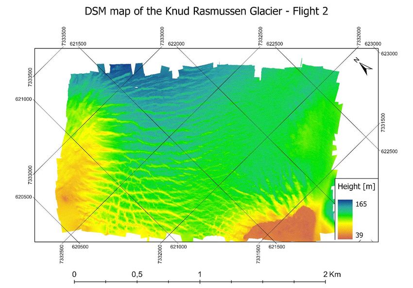
Preprints (www.preprints.org) | NOT PEER-REVIEWED | Posted: 1 December 2020                               doi:10.20944/preprints202012.0006.v1

                  case of a polar bear attack, we were equipped with a rifle. Fortunately, this did not happen. We were
                  aware that in the event of a drone crashing or losing control, we would lose the drone. It was not
                  possible to ascend the glacier, and the drone was moving at two kilometres. The landing site was too
                  small on the coastal stone moraine, but fortunately, the drone was not damaged.
                       We had two changeable cameras at disposal for the drone. Due to a malfunction of the RGB
                  camera, we used a NIR camera, which has a better passage of rays through the atmosphere and
                  better imaging, and in the end, it was also more suitable for capturing ice than an RGB camera
                  (glacier ice is off-white to light blue which is not perfect for image correlation used for image
                  processing). Using the drone eBee, two overflights of the same area were performed with a time
                  span of about 4 hours. During the first flight, a total of 162 NIR images were taken (Fig.8 b). During
                  the second flight, 170 NIR images were recorded. During the first flight, a signal was lost due a very
                  high rock cliff nearby by the last flight line; the drone emergency system interrupted the flight and
                  returned it to the take-off point.
                       The flight time took approximately 35-40 minutes at an altitude of 180 m. Due to the smaller
                  capacity of the batteries in the frost, we did not choose a lower flight or a longer flight. Another
                  problem was the high rocks on both sides of the glacier.
                       The last flight line was not fully completed, it was not the time to repeat flight and therefore the
                  second flight was slightly modified. The aim was to record both shores of the moraine, which could
                  not change in a few hours, unlike the movement of the glacier, which was supposed to be the largest
                  somewhere in the middle.

                                 Figure 7. Google Earth - processed satellite images (but the latest is from 2016).

                                         (a)                                                        (b)
                        Figure 8. (a) Flight No.1 (SenseFly eMotion 2; the map background was out of date and the flight
                        plan had to be estimated), (b) a typical photo using NIR camera Canon PowerShot ELPH 110 HS
                                                                      (NIR).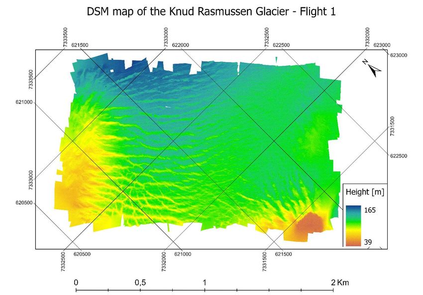
Preprints (www.preprints.org) | NOT PEER-REVIEWED | Posted: 1 December 2020                           doi:10.20944/preprints202012.0006.v1

                  2.4. Data processing
                       The data could only be processed in a laboratory at the University in Prague (not directly
                  during the expedition).
                       Data processing was performed by Agisoft Metashape program. The Highest setting was used
                  to orient the images. 74,416 tie points were found in the first set of images (sparse point cloud). In the
                  second set of images, the number of connecting points was 92,693. After the depth map was created,
                  221,341,562 points (dense point cloud) were created for the flight and 231,635,556 for the second
                  flight. Both point clouds were exported without modifying the coordinate systems.

                       Creating a point cloud, orthophoto, and DSM (digital surface model) was not a problem
                  (Fig.9-10); the problem was to calculate the movement of the glacier in two flights, it moves
                  nonlinearly (at the edges slowly and in the middle fastest). The difference in point clouds is usually
                  calculated in CloudCompare software; in this case, it simply did not work due to nonlinear motion.

                                    Figure 9. Flight No.1 and flight No.2 (orthophoto in near infrared range).

                                                     Figure 10. Flight No.1 and No.2 - DSM.

                        Accurately reference both point clouds from individual flights were a big problem. There were
                  no control points; it would be impossible to place them on the glacier. GNSS equipment on the drone
                  has an accuracy of 3-5m, which is not sufficient for this purpose. The assumption of movement in a
                  few hours was one to several meters maximally. The RTK system was not available and it would not
                  work here due to the short measurement time and conditions (no reference station was at disposal
                  too).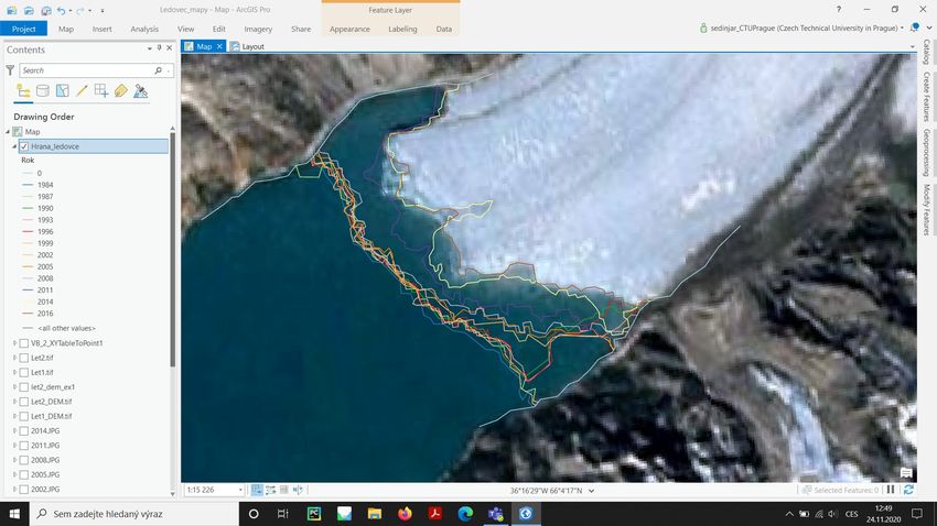
Preprints (www.preprints.org) | NOT PEER-REVIEWED | Posted: 1 December 2020                       doi:10.20944/preprints202012.0006.v1

                  2.5 Joining of both point clouds
                       Experiments were conducted to connect both point clouds from two overflights to each other
                  exactly. The first model was defined as a reference and the second was transformed into it. The
                  problem occurred with joining of the second point cloud with the tie points detected at the edge of
                  the model in a stone moraine. These found points were relatively stable and were used as fixed
                  points.
                       However, based on the unstable and inaccurately determined elements of internal and external
                  orientation (the drone has less than one kilogram and the flight is very affected by gusts of wind and
                  further camera used are low cost), the second model was joined with the reference one at their edge
                  excellent due to tie points, but in the middle, a model deformation has occurred and it reaches more
                  than 2m.
                       The software performs by joining a new calculation using the tie points as the control points
                  (points found on the first model, but only on edges of the model; in the middle of the glacier,
                  considerable movement is expected here and it is not possible to define high-quality fixed tie points)
                  and deforms the model by correcting the elements of external orientation during the new bundle
                  adjustment process. The model curls.
                       It was necessary to use a different procedure. Models cannot be joined only at fixed points or
                  control points at the edges of the model, because then an unknown deformation occurs in the middle
                  of the model. Both models were calculated separately, and the second model was joined only by a
                  similarity transformation (shifts, three rotations, scaling) using 6 tie points. It finally gave usable
                  results with an RMS of 0.67m.
                        A similarity transformation in 3D was used (Equation 1.):

                                                                                                                         (1)
                        where (X,Y,Z) are the final coordinates in the system of first model, (Xo, Yo, Zo) are the shifts, m
                  is the scale and (x,y,z) are the coordinates in second model.
                        The spatial seven-element transformation is given by seven unknowns, three translations, three
                  rotations and one scaling. The affine spatial transformation is similar to the seven-element
                  transformation, but it has nine unknowns, there are three scale values (there is a different scale for
                  each axis). To calculate the transformation key, it is necessary to calculate approximate values and
                  proceed this by iteration. However, in the case of incorrectly determined identical points, a problem
                  with the convergence of the calculation occurs. Both types of transformation are programmed in
                  Delphi, originally on the Faculty of Civil Engineering such as other university software for
                  geodetical using [23].

                       m is a scalar (similarity transformation) or M is a matrix (affine transformation, Equation 2.)

                                                                                                                         (2)

                       This result (RMS = 0.67m ) is acceptable due to the pixel size of 10 cm and the type and structure
                  of the surface, including possible actual deformation of the glacier over time. Better results cannot be
                  expected under the current conditions and used equipment. It should be noted that the model was
                  created from images taken in a time span of approximately 35 minutes. Even in this short time, parts
                  of the glacier probably moved.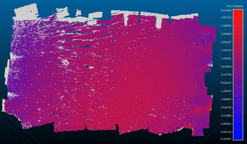
Preprints (www.preprints.org) | NOT PEER-REVIEWED | Posted: 1 December 2020                          doi:10.20944/preprints202012.0006.v1

                      Figure 11. Schematic deformation of both models after joining the point clouds with tie points, found
                                       at the edge of the model in a stone moraine (it should be stable).

                       Subsequently, both point clouds were spatially joined in the CloudCompare program. A total of
                  eight tie points (no exact control points measured with a precise GNSS devices were at disposal)
                  were used for identification and the total RMS was 0.67 m (Fig.11-12).

                                               Figure 12. Final RMS for both point clouds joining.

                  3. Data analyse
                       The next part was the analysis of the joined models and the search for real shifts in time. A
                  comparison of changes was performed using the Model-to-Model Cloud Comparison (M3C2)
                  method [24], (Fig.13). This is a method of calculating the distance between two clouds. The method
                  calculates distances only for so-called core points. This is the selection of a smaller sample of points
                  from the whole reference point cloud (however, the whole cloud is used for the calculation).
                       The points are usually selected based on the minimum distance they must contain. In the first
                  step, the normal vectors for each point are calculated. All points located at the maximum spherical
Preprints (www.preprints.org) | NOT PEER-REVIEWED | Posted: 1 December 2020 doi:10.20944/preprints202012.0006.v1
distance (s) specified by the user from the core points are used to calculate the normals. If the clouds
contain normal vectors from postprocessing, these normals can be used.
For each core point, a normal vector is calculated, which is the average of the normals of all
points that lie from the core point with the maximum distances. This vector forms the axis of the
cylinder. In the next step, a cylinder with a user-defined height (h) and radius (r) is interposed by a
cloud. The core point forms the centre of this cylinder. The position of a point is calculated as the
average of all points that are in this cylinder. A more detailed description of the method can be
found in Lague. et al. (2013) [25, 26], (Fig.14-15).
Figure 13. Model -to-Model Cloud Comparison (M3C2) method.
Figure 14. Graphical representation of the M3C2 distance.Preprints (www.preprints.org) | NOT PEER-REVIEWED | Posted: 1 December 2020 doi:10.20944/preprints202012.0006.v1
Figure 15. Histogram of the M3C2 distance.
Figure 16. Areas of significant change on the Knud Rasmussen Glacier in the time span four hours.
The results of the analysis show that the glacier moves fastest in the middle, which is not
surprising [27]. This result was expected, but it was about defining the average speed of movement
of the glacier. From the histogram of M3C2 distances, it can be concluded that (of course, with a
certain error up to about 0.7 m) the glacier Knud Rasmussen moves at an average speed probably
around 10 m per day. The fastest parts on Wednesday can have a speed over 15 m per day, while
the border parts move practically by this method immeasurably in the short time span (Fig.16).
4. Processing of historical aerial images
Thank to Anders Anker Bjørk (Dept. of Geoscience & Natural Resource Management
University of Copenhagen) we got a set of historical aerial images from the Danish Greenland
expedition (the seventh Thule Expedition 1932-33), (Fig.17).Preprints (www.preprints.org) | NOT PEER-REVIEWED | Posted: 1 December 2020 doi:10.20944/preprints202012.0006.v1
(a) (b)
Figure 17. (a) The Heinkel seaplane with open cockpit for three persons (pilot, radio-operator and
photographer in the back (photo The Arctic Institute, https://arktiskinstitut.dk/). Taking photos was
carried out from a height of up to 4500 meters at a temperature of -40 degrees Celsius frequently.
Nowadays, these conditions are hardly imaginable, (b) the Fairchild F-8 camera.
The set consist of several oblique aerial images in a form of scanned photo copies. After
searching on web, these original images were taken (probably) by the Fairchild F-8 photogrammetric
camera, which was released in 1930. Original images were taken probably on a film 5"x7", the focal
length was 240mm (12"). We only found this information about the photos. The fiducial marks were
very difficult to find and the frame data was unusable. It was uncertain whether the photographs
were complete in original format. Fortunately, the centre of the image was highlighted by a puncture
and a mark in the photographs. All scanned paper photocopies had to be transformed into detected
centres, fitted and cropped according to poorly visible fiducial marks to the same format. Projective
transformation was used, which got the best results.
Only eight historical images were selected, from which a project was created to process image
information into a 3D model. After many experiments, the project was successfully completed. It
was necessary to define at least basic parameters instead of elements of internal orientation. A focal
length of 240 mm was used, and the pixel size (14.2 µm) was derived from the size of the scanned
photographs and the original image size of 5´´by 5´´ (the additional part on film was used for frame
information as time, photo number etc.). Processing the data into a 3D model was difficult and
experimental. Metashape software was used. The first attempt at automatic processing was
unsuccessful, which was expected. It was necessary to the find suitable tie points manually; in the
end, 25 tie points were used for a correct calculation. A sparse cloud was calculated and the points
were filtered using gradual selection experimentally, the camera parameters were recalculated until
stable results were obtained, which - again only experimentally - were acceptable. The big problem
was that the pictures did not have a regular overlap, they were taken by hand and it was almost
always a pair of similar pictures. From the flight sequence of images of the Knud Rasmussen glacier,
all images were finally processed, but it must be said that the first two images were processed after
tens of attempt due a small overlapping. In the end, however, it can be said that we managed to
create a relatively good and illustrative model of a historical status (Fig.18-20).
The most interesting result is the fact that the face of the Knud Rasmussen glacier practically
changes very little compared to the dramatically receding other glaciers, including right next to the
mouth of the Karale glacier (the glacier on the left part of the model).Preprints (www.preprints.org) | NOT PEER-REVIEWED | Posted: 1 December 2020 doi:10.20944/preprints202012.0006.v1
Figure 18. The created 3D model of Karale (left) and Knud Rasmussen glacier mouths (right) with tie
points and photo positions; 1.23 million faces.
Figure 19. A detail of the 3D model – the Knud Rasmussen glacier in the 1930s.Preprints (www.preprints.org) | NOT PEER-REVIEWED | Posted: 1 December 2020 doi:10.20944/preprints202012.0006.v1
Figure 20. An orthographic view on the 3D model shows glacier faces; it can be joined with
satellite and drone images. Unfortunately, the images were taken as oblique which caused a
considerable amount of hidden parts due to perspective (white areas).
5. Landsat data
Google Earth provides previews of Landsat satellite data from 1984-2016 (Fig.21) for the Karale
and Knud Rasmussen glaciers. The data were always taken on the same day (directly on the last day
of the year, Dec 31st), which is an advantage for comparison. In ArcGIS all the images were
compared (Fig.22). It can be seen from the series of images that major changes to the front of the
Knud Rasmussen glacier did not occur until after 2000. The Karale glacier began to recede as early as
1990.
(a)
(b)
(c)
Figure 21. Landsat data from Google Earth, (a) from 1984, (b) from 2002, (c) from 2016.Preprints (www.preprints.org) | NOT PEER-REVIEWED | Posted: 1 December 2020 doi:10.20944/preprints202012.0006.v1
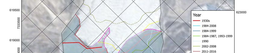
Figure 22. Landsat data from Google Earth, the Knud Rasmussen changes interpretation between
1984-2016 (until 2011 small changes only).
Figure 23. A final interpretation of glacier changes between 1932 and 2019.Preprints (www.preprints.org) | NOT PEER-REVIEWED | Posted: 1 December 2020 doi:10.20944/preprints202012.0006.v1
Table 1. The approximate changes of the Knud Rasmussen Glacier;
the basic state was the year 1984 - i.e. the state "zero".
Year Decrease [thousand m2]
1984 0
1932 -200*
1987 +10
1990 -204
1993 +200
1996 -80
1999 -50
2002 -230
2005 -410
2008 -495
2011 -700
2014 -234
2016 -207
2019 -967*
*interpolated, the data did not cover the entire glacier
Figure 24. The Knud Rasmussen Glacier changes between 1932 and 2019.Preprints (www.preprints.org) | NOT PEER-REVIEWED | Posted: 1 December 2020 doi:10.20944/preprints202012.0006.v1
Figure 25. The Knud Rasmussen Glacier in historical photo (detail); unfortunately, from this photo
cannot be possible to get 3D information (only the glacier delimitation).
In the 1930s, the condition of the glacier was the same as in the early new millennium until 2011.
This is quite clearly evident from the georeferenced orthophoto from the 1930s. The north-eastern
part of the glacier front was located at the position from 2002-2008. The front of the glacier from the
1930s was behind the front from 1984. But we do not know exactly when the flight was made, we
know that it was very likely in the Summer. The question is what the front of the glacier looked like
in the winter in the 1930s. Similarly, the data from 2019 are from a Summer that was warm (Fig.
23-25). Other satellite dates are always from winter.
5. Discussion and Conclusions
The research looked at the possibility of monitoring the flow rate of the Knud Rasmussen
glacier in eastern Greenland using RPAS based on tome changes detected from two overflights.
According to the available results, it can be stated that the most significant changes occur in the
middle part of the studied area. That was expected. The M3C2 distance histogram shows that the
changes rarely exceed three meters. A typical movement of the middle part of this glacier can be
between 1,5-2m in a time span 4 hours, it means 9-12m per day, which is acceptable. There is, of
course, a possible error of up to RMS 67cm, given the inaccuracy of joining both point clouds. In
conclusion, it can be stated that the use of a drone for monitoring the speed of movement of the
glacier is possible even after a relatively short time span. Of course, it depends on the type and
parameters of the glacier. The fastest running ones have a speed in the middle of up to tens of meters
per day (Egi glacier, Jakobshavn glacier, etc., Greenland). In the case of the Knud Rasmussen glacier,
the flow rate is considerable and can reach a value of around 12 m per day; however, this is only an
extrapolation. It is true that only a short time span was used, and the parameters of the flight were
not ideal due to the conditions and time problems. From the historical images, we can deduce that
the glacier recedes inland and its flow rate clearly increases, like most other glaciers. It is true that
the Knud Rasmussen glacier retreats into the inland not so progressively as by other glaciers, which
have moved backward on kilometres to inland due to climate change. An analysis of historical
images, satellite images and new drone images shows that the front of the Knud Rasmussen glacier
was practically in the same place from the 1930s until 2000. Only later the glacier began to recede.
Satellite data on the Google Earth is outdated for the area, with new drone images showing the
accelerated retreat of the glacier front in recent years. However, the newest (2019) and the oldest
(1932-1933) image data were obtained in the summer, whereas satellite data from Landsat were
always acquired on the last day of the year.Preprints (www.preprints.org) | NOT PEER-REVIEWED | Posted: 1 December 2020 doi:10.20944/preprints202012.0006.v1
Author Contributions: Conceptualization, K.P.; methodology, K.P and K.P. jr.; technical advisory and
supervision, K.P. and JŠ.; data processing, K.P., K.P. jr. and J.Š.; investigation, K.P.; writing—original draft
preparation, K.P.; writing—review and editing, K.P. jr. and J.Š.; visualization, K.P., K.P. jr. and J.Š.; project
administration, K.P.; All authors have read and agreed to the published version of the manuscript.
Funding: This research was funded by the Czech Technical University in Prague Grant number
SGS20/053/OHK1/1T/11 and the APC was funded by the Czech Technical University in Prague, FCE, dept. of
Geomatics”.
Acknowledgments: The project was funded partly by the Faculty of Civil Engineering, CTU in Prague for
university-specific research. Finally, we would like to thank Mr. Arved Fuchs and crew member Dagmar Aaen
for an incredible experience and perfect service and to Anders Anker Bjørk (University of Copenhagen) for the
photographs provided and the immediate and friendly response.
Conflicts of Interest: The authors declare no conflict of interest. The funders had no role in the design of the
study; in the collection, analyses, or interpretation of data; in the writing of the manuscript, or in the decision to
publish the results.
References
1. Cartographic expeditions to Greenland, (cited 10-11-2020)
https://en.wikipedia.org/wiki/Cartographic_expeditions_to_Greenland
2. Pickering, K. (Ed.) Amundsen. The International Journal of Scientific History, DIO Vol. 10, 2000, Triple Issue:
Copublished with the University of Cambridge Expansion of DIO Report to N.Y.Times Page One 1996/5/9.
http://www.dioi.org/vols/wa0.pdf
3. Běhounek, F. Trosečníci polárního more (Castaways of the polar sea). Albatros, Prague, 1955 (reprint 1989,
in Czech)
4. Slater, T.; Hogg, A.E.; Mottram, R. Ice-sheet losses track high-end sea-level rise projections. Nature Climate
Change, 1–3. 2020. ISSN 1758-6798. Retrieved 8 September 2020. https://doi.org/10.1038/s41558-020-0893-y
Mouginot, J.; Rignot, E; Bjørk, A.A.; Van den Broeke, M.; Millan, R; Morlighem, M; Noël, B; Scheuchl, B;
Wood, M. Forty-six years of Greenland Ice Sheet mass balance from 1972 to 2018. Proceedings of the
National Academy of Sciences. 2019, 116 (19) 9239-9244; https://doi.org/10.1073/pnas.1904242116,
https://www.pnas.org/content/116/19/9239
5. Encyclopædia Britannica. 1999 Multimedia edition, (cited 28-10-2020)
6. Greenland Rapidly Rising as Ice Melt Continues, 2020. www.miami.edu [online], (cited 2020-10-05),
http://www.miami.edu/index.php/news/releases/greenland_rapidly_rising_as_ice_melt_continues/
7. Houghton, J.E.T; Ding, Y.; Griggs, D.J.; Noguer, M.; van der Linden, P.J.; Dai, X.; Maskell, K.; Johnson, C.A.
(eds.), Climate Change 2001: The Scientific Basis. Contribution of Working Group I to the Third
Assessment Report of the Intergovernmental Panel on Climate Change (IPCC), 2001. Cambridge
University Press, Cambridge, United Kingdom and New York, NY, USA, 881pp. Archived from the
original on 2006-02-10.
https://www.researchgate.net/publication/216811760_Climate_Change_2001_The_Scientific_Basis
8. Sasgen, I.; Wouters, B.; Gardner, A.S.; King, M. D.; Tedesco, M.; Landerer, F.W.; Dahle, Ch.; Save, H.;
Fettweis, X. Return to rapid ice loss in Greenland and record loss in 2019 detected by the GRACE-FO
satellites. 2020. Communications Earth & Environment. 1 (1): 1–8.. ISSN 2662-4435. Retrieved 6 September
2020. https://doi.org/10.1038/s43247-020-0010-1
9. Fridtjof Wedel-Jarlsberg Nansen, https://en.wikipedia.org/wiki/Fridtjof_Nansen, (cited 10-10-2020)
10. Knud Rasmussen. https://alchetron.com/Knud-Rasmussen, (cited 10-10-2020)
11. Andrej Abplanalp, Swiss National Museum, Alfred de Quervain,
https://blog.nationalmuseum.ch/en/2020/02/de-quervain-greenland-1912/ (cited 10-10-2020)
12. Stephan Orth. Opas Eisberg. Auf Spurensuche durch Grönland. Spiegel Online. 2013, pp.251
13. Bjørk, A.A.; Kjær, K.H.; Larsen, N.K.; Kjeldsen, K.K.; Khan, S.A.; Funder, S.V.; Korsgaard, N.J. The
Greenland Ice Sheet - 80 years of climate change seen from the air. Natural History Museum of Denmark, Faculty
of Science, University of Copenhagen, 2014. 978-87-87519-46-5. 180pp.
14. Bjørk, A.A, Kjær, K., Korsgaard, N. et al. An aerial view of 80 years of climate-related glacier fluctuations
in southeast Greenland. Nature Geoscience, 5, 427–432. 2012. https://doi.org/10.1038/ngeo1481Preprints (www.preprints.org) | NOT PEER-REVIEWED | Posted: 1 December 2020 doi:10.20944/preprints202012.0006.v1
15. Raeva, P.; Pavelka jr, K.; Geospatial and temporal analyses of rural area for vegetation analysis. Civil
Engineering Journal; Prague Iss. 2, 2020. https://doi.org/10.14311/CEJ.2020.02.0021
16. Šedina, J.; Housarová, E.; Raeva, P. Using RPAS for the detection of archaeological objects using
multispectral and thermal imaging. European Journal of Remote Sensing. 2019, 52(sup1), 182-191. ISSN
2279-7254. https://doi.org/10.1080/22797254.2018.1562848
17. Korth, W.; Hoffman, U.; Hitziger, T.; Küchenmeister, T., Pawelka, K. Klimabedingte Veränderungen des
Inlandeises im südlichen Grönland, 19. Internationale Geodätische Woche Obergurgl. 2017. Berlin and
Offenbach: Herbert Wichmann Verlag, Wichmann Verlag. ISBN 978-3-87907-624-6.
18. Näcke, L., Vergleich kinematischer GNSS-Daten aus Ostgrönland (Comparison of kinematic GNSS data
from East Greenland), BTU Cottbus, Germany, Bachelor Thesis, 2020
19. Pavelka, K.; Šedina, J.; Matoušková, E.; Hlaváčová, I.; Korth, W. Examples of different techniques for
glaciers motion monitoring using InSAR and RPAS. European Journal of Remote Sensing. 2019, 52(1),
219-232. ISSN 2279-7254. https://doi.org/10.1080/22797254.2018.1559001
20. Bash, E.A.; Moorman, B.J.; Gunther, A. Detecting Short-Term Surface Melt on an Arctic Glacier Using
UAV Surveys. Remote Sensing. 2018, 10, 1547. https://www.mdpi.com/2072-4292/10/10/1547#
21. Zwally, J., Abdalati W., Herring,T.,Larson, K.,Saba,J., Steffen, K. Surface Melt-Induced Acceleration of
Greenland Ice-Sheet Flow Science. 2002. 297 (5579): 218–222. https://doi.org/10.1126/science.1072708
22. Štroner, M., Pavelka, K. Lineární prostorová transformace (Linear spatial transformation). In Czech.
Geodetický a kartografický obzor. 2001, Vol. 47, Nr. 3, p. 233-235. ISSN 0016-7096.
23. M3C2 (plugin). CloudCompare. (cited 10-10-2020)
https://www.cloudcompare.org/doc/wiki/index.php?title=M3C2
24. Lague, D.; Brodu, N.; Leroux, J. Accurate 3D comparison of complex topography with terrestrial laser
scanner: Application to the Rangitikei canyon (N-Z). ISPRS Journal of Photogrammetry and Remote
Sensing. 82. 2013. https://doi.org/10.1016/j.isprsjprs.2013.04.009
25. Barnhart, T.B.; Crosby, B.T. Comparing Two Methods of Surface Change Detection on an Evolving
Thermokarst Using High-Temporal-Frequency Terrestrial Laser Scanning, Selawik River, Alaska. Remote
Sensing. 2013, 5, 2813-2837. https://www.mdpi.com/2072-4292/5/6/2813#
26. The Greenland Ice Sheet 80 years of Climate change seen from the Air, (cited 20-10-2020),
https://www.youtube.com/watch?v=ygCKQZiOSNwYou can also read