DRIVE-BY LOCALIZATION OF ROADSIDE WIFI NETWORKS
←
→
Page content transcription
If your browser does not render page correctly, please read the page content below
Drive-by Localization of Roadside WiFi Networks
              Anand Prabhu Subramanian                 Pralhad Deshpande                     Jie Gao           Samir R. Das
                 Computer Science Department, Stony Brook University, Stony Brook, NY 11794-4400, USA
                                  Email: {anandps, pralhad, jgao, samir}@cs.sunysb.edu

   Abstract—We use a steerable beam directional antenna
mounted on a moving vehicle to localize roadside WiFi access
points (APs), located outdoors or inside buildings. Localizing APs
is an important step towards understanding the topologies and
network characteristics of large scale WiFi networks that are
deployed in a chaotic fashion in urban areas. The idea is to
estimate the angle of arrival of frames transmitted from the
AP using signal strength information on different directional
beams of the antenna – as the beam continuously rotates while
the vehicle is moving. This information together with the GPS
locations of the vehicle are used in a triangulation approach to
localize the APs. We show how this method must be extended
using a clustering approach to account for multi-path reflections
in cluttered environments. Our technique is completely passive
requiring minimum effort beyond driving the vehicle around
in the neighborhood where the APs need to be localized, and                        Fig. 1.    Drive-by localization of roadside APs.
is able to improve the localization accuracy by an order of
magnitude compared with trilateration approaches using omni-
directional antennas, and by a factor of two relative to other       manner. Many urban regions have a high density of WiFi
known techniques using directional antennas.                         APs – deployed in a “chaotic” fashion [7] in homes and
                                                                     businesses, in campuses and hotspots, or as a part of a
                      I. I NTRODUCTION                               metro or municipal WiFi effort [8]. There is little knowledge
   Localization of the nodes in a WiFi (802.11) network using        about the nature of these networks, e.g., density, connectivity,
radio-based information – such as signal strength, angle of          interference properties, etc. The first step in understanding
arrival (AoA) etc. – is an important problem. The simple             their nature is estimating locations of the APs. We expect that
reason for this is that devices with WiFi interfaces are ubiq-       at the minimum our effort will provide researchers significant
uitous and localization of wireless/mobile devices enables           datasets for simulations and modeling purposes. We hope
interesting applications. GPS receivers are not available with       that this will eventually lead to significant research as in
most wireless clients making radio-based localization the only       understanding Internet topology [9], [10] in wired networking
viable option. Needless to mention that GPS may not always           context. Other than datasets for research use, learning locations
work in indoors and in urban canyons.                                of APs may reveal interesting social aspects. We will show
   In the most common approach for radio-based localization          later the accuracy of our localization is good enough to
for WiFi, location-tagged RF fingerprinting is used for sig-         localize APs within the boundary of a typical house or even
nals from infrastructure nodes (i.e., access points or APs).         an apartment. This can lead to interesting data sets for social
This location information must be independently determined.          science – correlating census data (say, level of education or
RADAR [1] and many followup papers [2]–[4] have used                 home price) to Internet usage.1
this basic method for indoor localization. On the other hand,           While several war-driving databases are in existence [12]
Intel’s Place Lab work [5] used a similar approach for outdoor       [13], the location information therein is very primitive. The
localization. In a different approach called VORBA [6], rotat-       database simply contains the locations where the APs are heard
ing directional antennas are used in APs and a combination           with a sniffer. As we will show later, even with the most
of signal strength and AoA information is used to localize           sophisticated techniques this information can only provide
clients in indoor environments. VORBA does not require RF            very rough location estimates, with errors in hundreds of
fingerprints, but needs multiple APs with rotating directional       meters. Our goal here is to be able to improve such location
antennas. All these approaches have been primarily used for          estimates by an order of magnitude.
localizing wireless client nodes, and not the infrastructure.           In our approach, we exploit the M OBI S TEER architecture
   In this work, we consider the opposite problem – localiza-
tion of infrastructure nodes (APs). Our goal is to localize them        1 We are assuming that having an WiFi AP at home means that residents

in a passive fashion, i.e., without their direct participations      have broadband connection and use the Internet heavily. Note that we are
                                                                     ignoring privacy aspects. Our technique simply sniffs WiFi frames from streets
in the localization process. There are tremendous application        and public places. This is no different than Google’s Street View [11] that
for such localization. WiFi networks are growing in a viral          takes pictures from streets.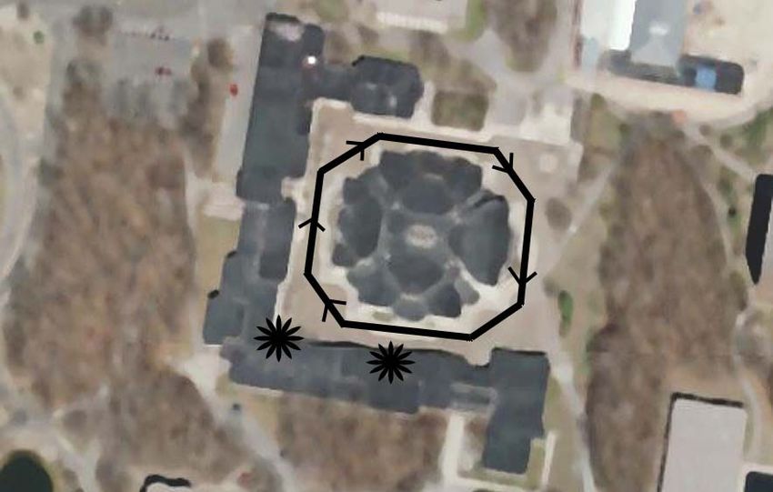
based on our recent work [14]. M OBI S TEER uses a steerable
beam directional antenna with a WiFi (802.11b/g) client
node mounted on a moving car. The antenna coupled with
appropriate protocols has been used to improve vehicular
connectivity to roadside APs [14]. Here, we use M OBI S TEER
to gather frames originating at roadside APs on different
directional beams to estimate the Angle of Arrival (AoA) of
the frames. For robustness reasons, our strategy requires that
many samples of AoA information be collected from different
                                                                                     (a)                              (b)
locations. Thus a moving car is indeed needed so that many
such samples can be collected with relatively little effort. The   Fig. 2. The beam patterns for phocus array antenna: (a) omni-directional;
                                                                   (b) two directional beams.
general idea is driving the car in the neighborhood where APs
need to be localized, and collecting GPS-tagged signal strength
                                                                   circle with 16 beam patterns. Figure 2 shows the manufacturer
information on different directional antenna beams for the
                                                                   provided beam patterns. We refer to the omni-directional beam
frames transmitted (e.g., beacons) by the APs. See Figure 1.
                                                                   with beam index 0 and the 16 directional beams we use
The approach is purely passive and based on “sniffing” alone;
                                                                   with beam indices 1 to 16. Adjacent beams are numbered
APs are unaware of the localization effort. Because of the use
                                                                   successively. We use a USB-based Garmin [22] GPS receiver
of a car, our work naturally targets outdoor use. However, the
                                                                   inside the car that is connected to the embedded computer. Our
APs can be anywhere – either indoor or outdoor. In fact, in
                                                                   experiments with this GPS receiver show a median position
most of our experiments they are indeed indoor.
                                                                   accuracy of about 5 meters. The entire hardware setup is called
   The rest of the paper is organized as follows. In Section II
                                                                   a M OBI S TEER node.
we describe our experimental platform and data collection
methods. In Section III we describe our localization approach.     B. Software Setup
The performance results are presented in Section IV. We               The madwifi driver allows creation of additional raw
follow it up with related work and conclusions.                    virtual interface (ath0raw) for a physical wireless interface.
     II. E XPERIMENTAL P LATFORM AND S CENARIOS                    The virtual interface allows reception of all 802.11 frames
                                                                   (control, management, data) as if in the monitor mode, while
A. Hardware Setup
                                                                   the main interface can still operate in the ad hoc or infrastruc-
   Our directional antenna setup uses electronically steerable     ture mode. We modified Kismet [23], a popular wireless packet
Phocus Array antennas from Fidelity Comtech [15] for the 2.4       sniffer software to optionally capture all packets received on
GHz band used in IEEE 802.11b/g. The Phocus Array antenna          the raw virtual interface. Kismet communicates with the GPS
system consists of eight element phased arrays driven by eight     server, running as a daemon (gpsd), and stamps the current
individual T/R (transmit-receive) boards that receive radio        time and GPS coordinates with each received frame from any
signals from the wireless card via an eight way RF splitter. The   AP.
phased arrays combine radio waves by introducing different            Each received frame (from APs) is also annotated with an
phase differences and gains in the eight arrays [16] [17]. A       index for the current beam pattern on the antenna, orientation
T/R board is essentially a vector modulator with bi-directional    of the car (more on this later) and the SNR (Signal to Noise
amplifier controlled by software. Various beam patterns are        Ratio). The SNR for each received frame is obtained from the
possible by setting the phases and gains in different boards       radio-tap header appended by the madwifi driver for each
differently.                                                       received frame. The AP’s identity (MAC address) is already
   The software control on the antenna to produce different        in the received frame. The tuple  is logged onto the flash memory of the Soekris
embedded computer (a Soekris net4511 board [18]). The beam         computer. We also refer to this as a measurement sample.
steering latency has been optimized to 250µs [14]. On the          SNR is represented in dB, given by 10 log(S/N ), where S
Soekris, we use a 802.11 a/b/g miniPCI card based on Atheros       and N are signal power received and noise floor respectively.
[19] chipset with an external antenna interface. The Soekris       In Atheros cards, the noise floor N is set at −95 dBm.
computer runs pebble Linux [20] with the Linux 2.4.26 kernel
and the widely used madwifi [21] device driver for the             C. Experimental Scenarios
802.11 interface.                                                     Figure 3 shows three representative environments in which
   While many beam patterns are possible using the phased          we did our experiments. It also shows the actual location of the
array, the manufacturer ships the antenna with 17 precomputed      APs and the driving path of the M OBI S TEER node. Figure 3(a)
patterns – one omnidirectional beam and 16 directional beams,      is a large open empty parking lot with no surrounding build-
each with an approximately 45◦ half-power beam-width and           ing.This scenario is used to demonstrate the performance of
low sidelobes. The directional gain is about 15dBi. Each direc-    our localization approach in an uncluttered environment and to
tional beam is overlapping with the next beam and is rotated       create a best case scenario. This is representative of relatively
by 22.5◦ with respect to the next, thus covering the 360◦          rural or empty environment.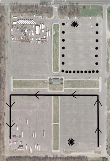
beam switching latencies can be ignored. We have fixed T
                                                                                to be 100 ms. This time is the default beacon period in
                                                                                most APs and also much longer than the switching latencies.
                                                                                Since T is not insignificant, it is not possible for a moving
                                                                                car to gather measurement samples on all beams exactly at
                                                                                the same location. Our experience has shown that so long
                                                                                as the measurement samples on all beams are within ‘close
                                                                                proximity’, the errors introduced are not significant in our
                                                                                technique. We have defined ‘close proximity’ as 5 m, which is
                                                                                similar to the GPS error bound for the GPS receiver we have
                                                                                used. We will discuss more about GPS errors in Section IV.
                                                                                   Still, the car must be driven very slowly. To see this,
                                                                                consider that an entire scan on 16 beams take 1.6 s. Thus,
       (a) Parking lot (2 APs).        (b) Apartment complex (17 APs).          the car should drive maximum 5 m in 1.6 s, i.e., 11.25 km/hr.
                                                                                Such slow driving may not always be practical. We propose
                                                                                to achieve the same effect by driving multiple times on the
                                                                                same route. This approach was also used in [14] to build
                                                                                up an RF signature database, though the context and use of
                                                                                the database were different. One simple approach to reduce
                                                                                the number of runs in the data collection process is to use
                                                                                multiple fixed directional antennas oriented along different
                                                                                directions connected to multiple radios on the moving vehicle.
                        (c) Office building (2 APs).                            This enables the vehicle to receive frames from APs in all
Fig. 3. Three experimental scenarios along with the AP locations and the
                                                                                directions throughout the drive.
driving trajectories. The black stars are the locations of the APs. The black      To summarize, the idea is to drive the car at normal speed
curve is the trajectory followed by the M OBI S TEER Node.                      appropriate for the roadway used. The drive is simply re-
                                                                                peated multiple times such that enough samples are collected.
   Figure 3(b) and 3(c) are complex environments where there                    Samples are then clustered such that samples taken within
are several two-storied buildings and large trees in close prox-                5 m from one another are assumed to be taken at the same
imity. They are the graduate student apartment complex and                      point P . P is assumed to be the centroid of the locations
the computer science department building in our university,                     of these samples that are in the cluster. For convenience we
respectively. The APs here are kept indoors as would be                         will refer to an instance of this point P as the measurement
normal in such environments. These are relatively challenging                   point. A larger number of samples naturally provide many such
scenarios for localization, as there are lots of possibilities of               measurement points along the roadway and provides better
reflections and shadowing. They are representatives of urban                    accuracy for localizing roadside APs. Average SNR is used in
homes and offices. The measurements reported here include                       the computation when there are multiple samples clustered
data collected from APs deployed in 21 different locations in                   on the same measurement point for the same beam. Here
the three scenarios shown in Figure 3.                                          also, larger number of samples provide better immunity from
                                                                                outliers due to fading. Later in Section IV, we will provide an
D. Data Collection                                                              analysis of sensitivity of our method to the number of samples
   Ideally, we would like to have measurement samples for                       as number of samples is directly related to the measurement
each AP on all beams at as many points on the roadway around                    effort.
the AP as possible. Samples on all beams let us estimate the                       To simplify the data collection process in the experimental
AoA – by comparing the received SNRs on all beams. In free                      results reported here, we have used a cart pushed at slow
space or relatively uncluttered environment, the beam with the                  walking speed in some instances (scenarios (a) and (c) in
highest SNR would be the one pointing towards the AP. A little                  Figure 3), instead of using a real vehicle and multiple drives.
variation of this also works well in cluttered environments with                This enabled us to collect sufficient number of samples per
reflections, which we will describe in the next section.                        AP on a single “walk”. This also enabled us to utilize walking
   The complexity in data collection comes from the fact that                   paths and open areas in the university campus where driving
we have a single radio and single antenna system in the                         is not allowed. For the experiments in scenario (b) in Figure 3,
M OBI S TEER node. The radio operates on a given channel and                    we drove at a very slow speed (approx 10 mph) and repeated
the antenna uses a given beam at a time. Thus, all channels                     the runs multiple times. About 40-60 measurement points are
and beams need to be scanned. However, for each channel and                     used to localize each AP in the experiments reported here.
beam combination the system must hold for certain duration                      We used our own APs for the experiments and made them
T , where T should be long enough to receive a frame from                       broadcast UDP packets at 250 packets/sec. This let us “speed
all APs in range and also long enough so that channel and                       up” the experiments as we could get many samples on the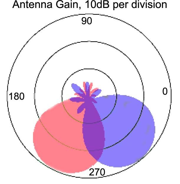
AP
Angular Error Zero Angular Direct signal
Angular Error
Error through wall
AP AP
Strongest Strongest Significant
beam beam obstruction
preventing Reflected
Measurement Measurement direct signal Signal
points points Measurement points
(a) (b) (c)
Fig. 4. (a) Angular error using center of directional beam. (b) Angular error considering beamwidth. (c) A scenario demonstrating reflection.
same beam for the same measurement point and used the plane for which the sum-square of the angular error from
average SNR for each combination. We used all the strongest beam directions is minimized similar to the
the same channel for all the APs. This speeds up the data approach used in [6]. See Figure 4(a). Two artifacts, however,
collection process further as multiple channels need not be complicate this scenario. They are described below.
scanned. Note that use of carts or UDP broadcast packets from • Non-zero beamwidth: The beams have non-zero width
AP are only used to reduce measurement effort and does not (about 45◦ between the half-power points on the main
have any fundamental impact on the results. lobe). Using the center of the beam for AoA calculations
may incur significant error; the non-zero beamwidth must
E. Determining Orientation
be accounted for. One way to account for this would
Since the antenna is mounted on the car in a fixed fashion, be to use angular error from the beam sides, i.e., the
the orientation of the car (with respect to some absolute ‘half-power’ directions, and pick the minimum of these
direction, say magnetic North) also provides an orientation two errors. In case the direction to the localized point
of the antenna setup. This ensures that the absolute direction is contained within the beam width, then the error is
of the directional beams can be determined by knowing the assumed zero. See Figure 4(b).
car’s orientation. Orientation of the car can be determined from • Reflections: In most realistic scenarios, radio obstructions
the heading computed from the GPS locations – a method and reflections would be present causing the strongest
commonly used in navigation systems. This, however, may beam point away from the AP. See Figure 4(c). This phe-
not provide enough accuracy for quick turns in small spaces. nomenon was quite evident in the measurements we did
For better accuracy, a digital compass such as [24] could be in [14] in cluttered environments (same as Figure 3(b)).
used.
In the experiments, we indeed used a compass – not B. Understanding and Modeling Reflections
digital, but a regular compass with a magnetic needle. During To understand the impact of reflections, we use Figures 5(a)
the walks for data collection, we manually ensured that the and (b) to show the measurement points (‘+’ symbols) and the
antenna setup is always oriented in the same direction. In direction of the strongest beam from each measurement point
the car experiments, GPS headings were used to compute the (arrows). For simplicity we are ignoring the beamwidth issue
orientation. We expect that use of digital compass will simplify for now and using the center of the beam for direction. The
the data collection process much and will likely provide better actual location of the access point is also shown (‘×’ symbols).
accuracy. These figures correspond to measurements for the empty
III. L OCALIZATION A LGORITHM parking lot (Figure 3(a)) and office building (Figure 3(c)), as
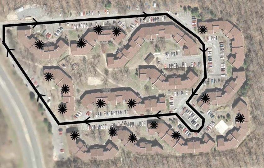
described in Section II-C. To complement these figures, we
A. Preliminaries also show the CDF of angular error of the strongest beam from
Our approach hinges on estimating the AoA of frames from the actual direction towards the AP from each measurement
a given AP at each measurement point. The AoA is estimated point (Figures 5 (c)).
by noting the average SNR for the frames from a given AP on Note that in the parking lot scenario most arrows are
each directional beam for the same measurement point. The pointing roughly towards the AP as expected. However, the
directional beam providing the strongest average SNR (we will behavior is quite different in the office building scenario. Most
call this the strongest beam) is expected to point directly to the of the arrows are pointing in a different direction, presumably
AP discounting reflections. Thus, the AoA can be estimated by due to reflections. Figure 5 (c) qualitatively demonstrates this.
determining the strongest beam and then using the orientation Note that for the parking lot scenario, the error CDF is rising
information (Section II-E) to determine the absolute direction sharply, and for the office building scenario, the rise is quite
of the strongest beam. (Unless mentioned otherwise, the beam gradual denoting significant errors. The median angular error
direction corresponds to the center of the beam.) Let α(i) for the parking lot is about 15◦ (small) and for the office
denote the absolute direction of the strongest beam at each building is about 55◦ (unacceptably large). Note also that the
measurement point (xi , yi ) along the drive. 90-percentile error for parking lot is 43◦ — similar to the
Let us first assume that signal reflections are not present. beamwidth of the antenna, while the 90-percentile error for
In this case, the AP can be localized at a point in the 2D office building is again very large (125◦ ).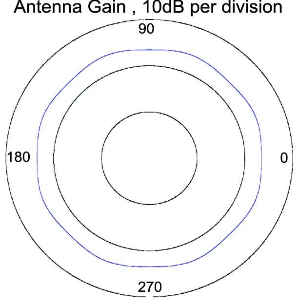
-20
                     Measurement points                                   Measurement points
-50                  Actual AP Location                                   Actual AP Location                    1
                                                                                                              0.9
  0                                                       0
                                                                                                              0.8
 50                                                                                                           0.7
                                                         20                                                   0.6

                                                                                                        CDF
100                                                                                                           0.5              Parking lot
                                                                                                              0.4          Office building
150                                                      40
                                                                                                              0.3
200                                                                                                           0.2
                                                         60                                                   0.1
250
                                                                                                                0
300                                                      80                                                         0         45       90      135      180
  -200 -150 -100 -50       0    50    100   150   200         -20     0       20        40      60              Absolute angular error(degree)
                   (a) Parking lot.                                   (b) Office building.                              (c) CDF of the angular error.
Fig. 5. (a), (b): AP location and directions of the strongest beams in two scenarios demonstrating the impact of reflections. (c): CDF of the angular error
of the strongest beam from the actual direction towards the AP in two scenarios.

   This study indicates that straight-forward approaches to                       In addition, we use weights when minimizing the sum-
minimize the sum-square of angular errors [6] using the                        square of angular errors. The intuition for this is as fol-
estimated AoA values can give rise to significant errors in                    lows. Since the strongest beam is the one that is important
cluttered environments where the strongest signal reaches the                  for estimating AoA, we should make distinctions between
M OBI S TEER node after one or more reflections. Since this                    measurement points with high SNR on the strongest beam
situation will be the common case for roadside APs, modeling                   compared to those with low SNR on the strongest beam.
reflections is important.                                                      We use the average SNR (in dB) of packets received in
   An interesting observation in Figure 5(b) is that while                     the strongest beam as the weighting function. This intutively
arrows are all pointing to different directions, there seems                   puts emphasis on measurement points close to the actual AP
to be a clustering effect. The arrows are not pointing to                      location or on those received on a direct beam.
random directions but towards one of a handful of possible                        More formally, let wi be the weights assigned to each
directions. This is as if each arrow is pointing towards either                measurement point. Let αl (i) and αr (i) denote the left and
the real AP or one of its images arising out of presence of                    right half-power directions of a beam with absolute angle
reflections. The complexity of modeling reflections now is                     α(i). We seek to find a k-clustering of the measurement
that there is no knowledge of the number and locations of                      points into k clusters (S1 , ..., Sk ) and obtain k locations
reflective surfaces that give rise to these images. Thus, there                Li = (Xi , Yi ), 1 ≤ i ≤ k, that minimize the following
is no knowledge of number of images to look for, and the real                  objective function:
AP is indistinguishable from any of its image.                                   k
   We will approach this problem in the following fashion.                         i=1   j∈Si   wj · min{[αl (j) − arctan(Yi − yj , Xi − xj )]2 ,
                                                                                                [αr (j) − arctan(Yi − yj , Xi − xj )]2 }
   1) Use the well-known k-means algorithm [25] to group the
      measurement points into k clusters such that each group                  Note that the quantity within {.} is the angular error using
      of measurement points have the strongest beam pointing                   the non-zero beamwidth idea. Since the angular error can be
      (approximately) towards the same location. These k                       between 0 and π, if the quantity within {.} is larger than π,
      locations include the real location and the images of                    it is subtracted from 2π.
      the AP. Since the number of reflective surfaces are not                     The k-means clustering algorithm works in the following
      known a priori, we use the Anderson-Darling normality                    way. For any given value of k, assume L1 , . . . , Lk are the k
      test [26] to learn the value of k while clustering (more                 locations of the AP (i.e., real and the images) to be deter-
      on this in section III-E).                                               mined. Initially, Li ’s are chosen randomly within the ‘feasible
   2) Determine which one of these k images is the real AP.                    region’.2 Each measurement point is mapped to some Li that
      We show that it is impossible to determine in a general                  provides the minimum angular error for this measurement
      case, but heuristics can be used quite successfully.                     point. Thus, the measurement points are now clustered into
We describe the details in the following subsection.                           k clusters. The algorithm then repeats the following two steps
                                                                               until convergence.
C. Modeling Reflections by k-Means Clustering                                      •   Compute a point for each cluster, denoted by Ci , in the
   Given the set of tuples < xi , yi , α(i) > for each mea-                            feasible region that minimizes the weighted intra-cluster
surement point along the drive, the main idea is to cluster                            sum-square of the angular errors within each cluster.
the measurement points into k clusters and find k locations
                                                                                 2 In our experiments, we defined the feasible region as a square of side
which minimize the aggregate of intra-cluster sum-square of
                                                                               600m around the measurement points. We assume the transmission range of
angular errors. The angular error is the error considering the                 the AP is not more than 300m and thus the possible location of the AP should
beamwidth and is determined as described in Section III-A                      be within a region of radius 300m from the measurement points.
• Ci ’s now become new Li ’s. Re-cluster by mapping each -45
measurement point to the Li that provides the minimum
-55
-55
RSS (dBm)
RSS (dBm)
angular error as before. -65 -65
Convergence is obtained when the clustering does not change. -75
-75
Now we have k locations, L1 , . . . , Lk , which represent the 2
-85
2
R = 0.559757 R = 0.335438
images of the AP including the real location. The next step is -85 -95
to choose one of these k points as the estimated location of
1.5 1.6 1.7 1.8 1.9 2 2.1 0.4 0.6 0.8 1 1.2 1.4 1.6 1.8 2
Log10(Actual Distance) Log10(Actual Distance)
the AP. (a) (b)
Fig. 7. Relationship between distance and RSS in (a) parking lot (b)
D. Choosing Real AP Location from k Images apartment complex.
The k-means clustering gives a set of possible locations of
the AP, with one of them being the true location and the rest data as there is no a priori knowledge of number of images.
of them reflected images. However, it is hard to distinguish Intuitively, we would like the measurement points to be
the true location from the image. A simple example is shown clustered nicely such that in each cluster the strongest beams
as in Figure 6. In the left figure, two measurement points all point to the same location Li . In other words, the angular
A, B receive signal from the AP. The signal from AP to B is error within one cluster should be uni-modal. Thus, we use the
direct but the signal to A was reflected once. Thus at location idea from the G-means algorithm [27] and learn the number
A the strongest beam points to the image of the AP. Notice of clusters, k, by checking whether the angular error values
that in this figure everything is symmetric, thus we can swap in each cluster follows a Gaussian distribution.
the AP and its image and have another feasible configuration We start with the value of k=1 and successively increment
(right). In other words, given a set of k possible locations k, performing a k-means clustering in each step as described
including the AP and its images, and the way the strongest before. After clustering, we check whether the error values
beam at each measurement point points to these locations, it in each cluster satisfy a statistical test for normality. If they
is impossible to tell the true location of the AP apart from do, we stop the procedure; otherwise, we increment k and
the images, as the same information may admit two (or more) repeat. We have used the standard Anderson-Darling normality
feasible configurations. test [26] [28] with a significance level3 of 1% to test for
normality.
1
0 1
0
AP
0
1
0
1
Image Image
0
1
0
1
AP
0
1
0
1 0
1
0
1
IV. P ERFORMANCE E VALUATION
0
1 0
1
0
1
0
1 0
1
0
1 In this section, we present a detailed performance evaluation
0
1 0
1
0
1
0
1 0
1
0
1
of our Drive-by Localization approach (DrivebyLoc) using
A 0
1 B A 0
1 B measurements from the 21 APs in three environments as
shown in Figure 3. The main comparison points are (i) a
Fig. 6. It is impossible to tell the true location of the AP apart from trilateration approach using distance information [29] esti-
the images, as the same information may admit two (or more) feasible mated using from signal strength information (SNR) using
configurations. omni-directional antenna,4 and (ii) VORBA [6], a localization
approach using directional antenna and AoA information. We
With this difficulty in mind, we use a heuristic to choose the also study and quantify the effect of several factors that impact
true AP location. Notice that if the strongest beam at a point P the performance of our system.
points to an image, then the image is always farther away from A. Benefit of Using Directional Antennas and AOA
P than the true location. Thus from a particular measurement
point’s view, the true location must be closer than any of In Figure 9 (a), we show the CDF of the localization errors
the images. Based on this observation, we propose a simple for DrivebyLoc and the trilateration approach for the 21 cases
heuristic that works very well in practice. Each measurement studied. The trilateration approach fundamentally depends on
point ranks the k images based on their distances to itself. The deriving distance estimates from the received signal strength
nearest image is ranked 1st and the next is ranked 2nd and (RSS). RSS is derived from SNR assuming constant noise. A
so on. We compute the weighted (weights being wj ’s defined simple propagation path loss modeling approach was used to
before) sum of the ranks for each image and choose the image infer distance from RSS following the method used in [30].
with the least value of the weighted sum. In our experiments The idea is to assume exponential decay of RSS with distance.
this always gives the location closest to the true AP location. Thus, RSS (in dBm) should have a linear relationship with
the log of distance. tuples are collected in
E. Learning k for Clustering the data collection phase assuming that the AP locations are
One remaining issue is to determine the right value of k 3 Significance level is the chance of incorrectly judging a set of values to
to be used in the k-means clustering algorithm. We need be not Gaussian.
some statistical means to estimate k from the measurement 4 The same antenna with omni-directional beam is used for this study.Localization Error (meters)
120
100 DrivebyLoc with beamwidth
DrivebyLoc without beamwidth
80 VORBA
60
40 (a) (a) (c) (c)
20
0
1 2 3 4 5 6 7 8 9 10 11 12 13 14 15 16 17 18 19 20 21
K=1 K=2 K=3 K=4
Fig. 8. Comparison of DrivebyLoc and VORBA.
known. This provides the scatterplot in Figure 7. A linear for DrivebyLoc is about 15 m, while for VORBA it is about
regression (shown) provides the necessary path loss model to 30 m.
be used to estimate distance from RSS. Note that (i) the R2 For the curious reader, we make a note here which scenarios
value of the regression is not high; and (ii) the parking lot these 21 sets of experiments correspond to. Note the labels
scenario provides a relatively more accurate modeling (higher (a) and (c) on top of some of the columns. These correspond
R2 ). The latter is likely due to lesser reflections and shadowing to scenarios Figure 3(a) and (c). The rest correspond to the
problems. scenario in Figure 3(b). Thus, as expected all schemes get the
Figure 9 (a) clearly shows that DrivebyLoc is about an order best results in the parking lot.
of magnitude better than trilateration. The median localization
C. Impact of GPS Accuracy
error in DrivebyLoc is about 15 m, while it is about 128 m
in trilateration. In fact, the maximum error in DrivebyLoc is As we take measurements while moving in a car, the loca-
less than 30 m. This shows that it can localize APs within tion of a measurement point is obtained through a GPS unit.
the accuracy of individual homes even in a very cluttered GPS devices are known to have errors [31]. In this section, we
environment. study the impact of GPS error in our localization approach. In
order to quantify the effect of GPS error, we did an experiment
B. Benefit of Modeling Reflection Using Clustering in a open parking lot as shown in Figure 3(a) by manually mea-
suring the distance between pairs of measurement points and
We now study the benefit of modeling reflection using finding absolute coordinates for each point. For this purpose,
the k-means clustering idea and also of modeling non-zero we used the cart setup as mentioned in Section II-D instead
beamwidth. For this purpose, we compare our results with of a car. We moved the cart and stopped at fixed measured
those of VORBA [6]. In VORBA a similar approach is taken, distances and took measurements on all directional beams.
except that a) signal reflections and b) non-zero beamwidth The dotted lines in Figure 3(a) show the points where the
are not modeled and c) no weighting using SNR is used. measurements were taken. We also noted the GPS coordinates
Figure 8 shows the localization errors obtained using three at each measurement point. The localization error for this
approaches in each of our 21 experiments categorized by the particular experiment using the manually measured absolute
value of k learned using the Anderson-Darling normality test. coordinates is around 12.6 m while the localization error using
For DrivebyLoc we show the performance with and without the GPS coordinates is around 16.4 m. This shows that the
modeling of non-zero beamwidth as discussed in Section III-A. GPS errors indeed worsen the performance of our localization
Note that the same results for DrivebyLoc with beamwidth approach. To get a better insight about the GPS accuracy, we
modeling was shown before in Figure 9(a) in CDF form. show the CDF of GPS errors for this particular experiment
Note that all three schemes perform almost similarly when in Figure 9 (b). The GPS error is computed by finding the
K = 1. VORBA’s performance worsens for larger K. Some difference between actual distance between two points and
very large errors are observed for VORBA K = 4 relative to to the distance computed using the GPS coordinates of the two
DrivebyLoc. This indicates the modeling reflections is critical points. The median GPS error is about 1.25 m and this causes
for accurate localization. The impact of modeling beamwidth an increase in our localization error by about 4 m.
is usually small and in general it is beneficial, though a few The GPS error could be higher in a cluttered environment
outliers are indeed noticed. But overall it should be recom- with buildings and trees blocking the GPS signals from
mended that DrivebyLoc be used with modeling beamwidth. the satellites. To understand this better, we repeated similar
Note also that DrivebyLoc’s performance with increasing K GPS error measurements for the office building scenario. As
is relatively stable compared with VORBA. Overall it can be expected, the errors were higher (median error about 5.5 m)
concluded that out of the three differences (see above) between Figure 9 (b), shows the CDF of GPS errors in these two sce-
DrivebyLoc and VORBA, modeling reflections has the most narios. This error is quite comparable to the errors DrivebyLoc
impact. Also, overall with the entire data set the median error has in the same scenario (about 20 m). It remains unclear howthe GPS errors are contributing to our localization errors. But approach to find the position of the wireless clients. Our
given the parking lot experience above, the results presented approach compared to VORBA is more robust to AoA in-
in Figure 8 likely underestimates DrivebyLoc’s performance. formation suffering from reflections in cluttered environments
that are representative of most urban WiFi deployments.
D. Impact of Car Speed There have been approaches for indoor localization using
As mentioned in Section II-D, the number of measurement other mediums such as ultra sounds, infrared, optical waves
samples could impact the accuracy of DrivebyLoc. The num- ets. Active Badge [32] is an indoor localization system that
ber of samples is inversely proportional to the car speed and employs infrared medium. Each user is given an infrared badge
directly proportional to the number of runs. Recall that in our and can be localized by IR stations that read the badges. Active
data collection approach we either used a car with slow drive Bat [33] uses a similar idea but employs ultrasound medium
(10 mph) or used a cart to walk. Also, in order to ’speed up’ and has extremely high accuracy in the order of centimeters.
the experiments we had the APs broadcast UDP packets at The Cricket [34] system from MIT is another indoor posi-
250 packets/sec which might happen in practise. We are now tioning system that uses ultrasound combined with RF. It uses
interested in evaluating what would happen if the car is driven several beacons that transmit ultrasound waves deployed in
at a more normal speed and APs do not transmit any frame the ceiling of each room in the building. The mobile nodes
other than beacons at 100ms intervals. We use our existing data receiving these waves infer the range and localize themselves.
to ‘simulate’ data collection at different speeds and then repeat In [35], Nasipuri and El Najjar propose an angle based indoor
it to simulate multiple runs. To do this simulation experiment, localization system employing optical waves. They use three
the existing data is laid out on an imaginary 2D map as points, rotating optical beacon signal generators that generate regu-
with each point as if ‘lit up’ at 100 ms intervals to simulate lar beacons and wireless sensor nodes equipped with photo
the corresponding AP beacons. An imaginary car is driven on sensors determine their locations from the estimated angular
the same roadway with slightly randomly varying speed (to separations between the optical sources. This idea is somewhat
simulate reality) about an average. Any point lit up within related our approach in the sense that they also use directional
5 m from the current car location is counted as measurement beams and angle information.
at the car location. This can be repeated to simulate multiple Finally, localization in multihop adhoc and sensor networks
drives. has been studied in a number of works [29], [36]–[38] and they
In Figure 9 (c), we show the mean localization errors for differ from each other depending on the type of information
the 17 experiments in the apartment complex scenario along used for localization such as angles, ranges and connectivity.
with the 95% confidence intervals. Two different speeds and The idea is to come up with a consistent embedding of the
multiple drives are shown. As expected, more runs and slower multihop network in either 2D or 3D plane.
speeds provide better mean localization error and smaller con-
fidence intervals. As discussed in Section II-D, use of multiple VI. C ONCLUSIONS
directional antennas and multiple radios on the moving vehicle In this paper, we have proposed and tested with abundant
would help to reduce the number of runs significantly. experiments a system with directional antennas for localizing
roadside WiFi access points, by simply driving through the
V. R ELATED W ORK neighborhood where the APs need to be localized. The power
RADAR [1] is one of the first systems to do indoor localiza- of the technique is its complete passive nature. It also does
tion of WiFi clients. The key idea is to do an RF fingerprinting not depend on any prior collection of RF fingerprinting data.
a priori to collect signal strength values from different APs While similar approaches have been investigated before [6],
tagged with location information. When the wireless client our major contribution is identifying that signal reflections
needs to be localized, it uses the current signal strength values can cause significant localization errors and then developing
it receives from different APs and do a lookup on the RF a clustering method to solve this problem. The idea is to
fingerprints. There are several follow up works similar to recognize a priori that there could be images of the AP, and
RADAR [2]–[4]. In particular, Ladd et al [2] improve the the real AP might be indistinguishable from the images. Thus,
accuracy of indoor localization from about 10 m by RADAR to we localize these – possibly multiple – images and then use a
within 1 m by using probabilistic inference of positions from heuristic to identify the real one among the set of images. The
noisy signal information. Using a similar idea, Intel’s Place method has demonstrated very satisfactory localization accu-
lab work [5] localize wireless clients in outdoor settings. All racies even in complex environments, compared with existing
these ideas suffer from the problem of carefully conducting approaches with omni-directional or directional antennas. In
RF fingerprinting. Also in these works, the emphasis is on spite of using the toughest scenarios for localization, the
localizing WiFi clients unlike our approach. localization errors are roughly between 10-30 m in spite of
Use of directional antennas for localization is not new. the fact many of our APs were indoors. This is very good
VORBA [6], one of the significant work in AoA based indoor compared to the localization error observed in Intel Place
WiFi localization uses WiFi APs equipped with a rotating Lab outdoor localization effort [5], where the median error is
directional antenna and estimates AoA information from pack- between 13-40 m in spite of very careful radio fingerprinting
ets transmitted from clients and uses a simple triangulation of the environment. This is an impressive performance givenLocalization Error (m)
1 1 50
20Mph
0.9 0.9 40Mph
0.8 0.8 40
0.7 0.7
0.6 0.6 30
CDF
CDF
0.5 0.5 Parking lot
0.4 0.4 Office building 20
0.3
0.3 DrivebyLoc
Trilateration 0.2 10
0.2
0.1
0.1
0
0 50 100 150 200 250 300 0 1 2 3 4 5 6 7 8 8 16 24 32
Localization error (meters) GPS error (meters) Number of Runs
(a) (b) (c)
Fig. 9. (a) Localization errors for DrivebyLoc and trilateration.(b) CDF of the GPS errors in two scenarios. (c) Impact of speed and number of runs on
localization error.
that we observed up to about 7.5 m of GPS error in similar [15] “802.11 Phocus Array Antenna System by Fidelity Comtech,”
environments. http://www.fidelity-comtech.com/.
[16] J. H. Winters and M. J. Gans, “Versus Phased Arrays in Mobile Radio
While the work so far is limited to 2D, this can be extended Systems,” IEEE Transactions on Vehicular Technology, vol. 48, no. 2,
to 3D using a combination of antennas so that directivity is pp. 353–362, 1999.
on both horizontal and vertical axes can be obtained. We will [17] Phocus Array Antenna System: Manual, Fidelity Comtech Inc. 2006.
[18] “Soekris Engineering,” http://www.soekris.com/.
consider this in the future. We expect that an important fallout [19] “Atheros Communications,” http://www.atheros.com.
of our work will be the creation of a very accurate ‘WiFi map’ [20] “NYCwireless Pebble Linux,” http://www.nycwireless.net/pebble.
of urban APs with a minimum effort, and eventually motivate [21] “MADWiFi Project,” http://sourceforge.net/projects/madwifi/.
[22] “Garmin GPS System,” http://www.garmin.com/.
novel applications. [23] “Kismet Wireless,” http://www.kismetwireless.net/.
[24] “Honeywell HMC6352 Digital Compass Solution,”
ACKNOWLEDGMENT http://www.ssec.honeywell.com/magnetic/datasheets/HMC6352.pdf.
Anand Prabhu Subramanian, Pralhad Deshpande and Samir [25] J. B. MacQueen, “Some Methods for classification and Analysis of
Multivariate Observations,” in 5th Berkeley Symposium on Mathematical
Das’s research has been partially supported by the NSF Statistics and Probability, Berkeley, University of California Press, 1967.
grants CNS-0519734 and CNS-0721455. Jie Gao would like [26] T. Anderson and D. Darling, “Asymptotic theory of certain ’goodness-
to acknowledge the support of NSF CAREER Award CNS- of-fit’ criteria based on stochastic processes,” Annals of Mathematical
Statistics, vol. 23, pp. 193–212, 1952.
0643687. [27] G. Hamerly and C. Elkan, “Learning the K in K-mean,” Advances in
Neural Information Processing Systems (MIT Press), vol. 16, 2004.
R EFERENCES [28] M. Stephens, “EDF Statistics for Goodness of Fit and Some Compar-
isons,” Journal of the American Statistical Association, vol. 69, pp. 730–
[1] P. Bahl and V. N. Padmanabhan, “RADAR: An in-building RF-based
737, 1974.
user location and tracking system,” in IEEE INFOCOM, 2000, pp. 775–
[29] A. Savvides, C.-C. Han, and M. B. Srivastava, “Dynamic fine-grained
784.
localization in Ad-Hoc networks of sensors,” in ACM MOBICOM, 2001,
[2] A. M. Ladd, K. E. Bekris, A. Rudys, G. Marceau, L. E. Kavraki,
pp. 166–179.
and D. S. Wallach, “Robotics-based location sensing using wireless
[30] J. Camp, J. Robinson, C. Steger, and E. W. Knightly, “Measurement
ethernet,” in ACM MOBICOM, Atlanta, GA, September 2002.
Driven Deployment of a Two-Tier Urban Mesh Access Network,” in
[3] P. Krishnan, A. S. Krishnakumar, W.-H. Ju, C. Mallows, and S. Ganu, “A
MOBISYS, Uppasala, Sweden, June 2006.
system for LEASE: System for location estimation assisted by stationary
[31] GPS Errors and Estimating Receiver Accuracy, http://edu-
emitters for indoor RF wireless networks,” in IEEE Infocom, Hongkong,
observatory.org/gps/gpsaccuracy.html.
March 2004.
[32] R. Want, A. Hopper, V. Falcao, and J. Gibbons, “The active badge
[4] M. Youssef, A. Agrawala, and U. Shankar, “WLAN location determina-
location system,” ACM Transactions on Information Systems, vol. 10,
tion via clustering and probability distributions,” University of Maryland,
pp. 91–102, January 1992.
College Park, MD, Tech. Rep., March 2003.
[33] A. Harter, A. Hopper, P. Steggles, A. Ward, and P. Webster, “The
[5] Y.-C. Cheng, Y. Chawathe, A. LaMarca, and J. Krumm, “Accuracy
anatomy of a context-aware application,” in ACM MOBICOM, Seattle,
characterization for metropolitan-scale wi-fi localization,” in MOBISYS,
Washington, August 1999.
2005, pp. 233–245.
[34] N. Priyantha, A. Miu, H. Balakrishnan, and S. Teller, “The cricket
[6] D. Niculescu and B. Nath, “VOR Base Stations for Indoor 802.11
compass for context-aware mobile applications,” in ACM MOBICOM,
Positioning,” in ACM MOBICOM, 2004.
Rome, Italy, July 2001.
[7] A. Akella, G. Judd, P. Steenkiste, and S. Seshan, “Self Management
[35] A. Nasipuri and R. E. Najjar, “Experimental Evaluation of an Angle
in Chaotic Wireless Deployments,” in ACM MOBICOM, Cologne,
Based Indoor Localization System,” in WiNMee, Boston, MA, April
Germany, August 2005.
2006.
[8] “Chaska wireless solutions,” http://www.chaska.net/.
[36] D. Niculescu and B. Nath, “Ad hoc positioning system (APS),” in IEEE
[9] M. Faloutsos, P. Faloutsos, and C. Faloutsos, “On power-law relation-
Globecom, November 2001.
ships of the Internet topology,” Proc. Sigcomm, pp. 251–262, 1999.
[37] J. Bruck, J. Gao, and A. Jiang, “Localization and Routing in Sensor
[10] D. Alderson, L. Li, W. Willinger, and J. Doyle, “Understanding Internet
Networks by Local Angle Information,” in ACM MOBIHOC, May 2005.
topology: principles, models, and validation,” IEEE/ACM Transactions
[38] L. Girod and D. Estrin, “Robust range estimation using acoustic and
on Networking, vol. 13, no. 6, pp. 1205–1218, 2005.
multimodal sensing,” in International Conference on Intelligent Robots
[11] “Google Street View,” http://maps.google.com/help/maps/streetview/.
and Systems, October 2001.
[12] “WiFi Maps,” http://wifimaps.zhrodague.net/.
[13] “Wireless Geographic Logging Engine (WIGLE),”
http://www.wigle.net/.
[14] V. Navda, A. P. Subramanian, K. Dhanasekaran, A. Timm-Giel, and
S. R. Das, “MobiSteer: Using Steerable Beam Directional Antenna for
Vehicular Network Access,” in MOBISYS, San Juan, Puerto Rico, June
2007.You can also read