The importance of corner sharpness in the BARC test case: a numerical study
←
→
Page content transcription
If your browser does not render page correctly, please read the page content below
The importance of corner sharpness
                                                                    in the BARC test case:
arXiv:2109.03522v1 [physics.flu-dyn] 8 Sep 2021

                                                                       a numerical study
                                                                    Alessandro Chiarini, Maurizio Quadrio
                                                      Politecnico di Milano, Dept. Aerospace Science and Technologies
                                                                                     September 9, 2021

                                                                                              Abstract
                                                             The BARC flow is studied via Direct Numerical Simulation at a relatively low
                                                        turbulent Reynolds number, with focus on the geometrical representation of the
                                                        leading-edge (LE) corners. The study contributes to further our understanding of
                                                        the discrepancies between existing numerical and experimental BARC data. In a
                                                        first part, rounded LE corners with small curvature radii are considered. Results
                                                        show that a small amount of rounding does not lead to abrupt changes of the mean
                                                        fields, but that the effects increase with the curvature radius. The shear layer sep-
                                                        arates from the rounded LE at a lower angle, which reduces the size of the main
                                                        recirculating region over the cylinder side. In contrast, the longitudinal size of the
                                                        recirculating region behind the trailing edge (TE) increases, as the TE shear layer
                                                        is accelerated. The effect of the curvature radii on the turbulent kinetic energy
                                                        and on its production, dissipation and transport are addressed. The present results
                                                        should be contrasted with the recent work of [37], who found via implicit Large-
                                                        Eddy Simulations at larger Reynolds numbers than even a small curvature radius
                                                        leads to significant changes of the mean flow.
                                                             In a second part, the LE corners are fully sharp and the exact analytical solu-
                                                        tion of the Stokes problem in the neighbourhood of the corner is used to locally
                                                        restore the solution accuracy degraded by the singularity. Changes in the mean
                                                        flow reveal that the analytical correction leads to streamlines that better follow
                                                        the corners. The flow separates from the LE with a lower angle, resulting in a
                                                        slightly smaller recirculating region. The corner-correction approach is valuable
                                                        in general, and is expected to help developing high-quality numerical simulations
                                                        at the high Reynolds numbers typical of the experiments with reasonable meshing
                                                        requirements.

                                                  1    Introduction
                                                  The flow around bluff bodies with sharp corners is interesting for both fundamental
                                                  research and industrial applications, particularly in civil engineering. The rectangular
                                                  cylinder is a simple yet representative prototype of such bodies. Despite the simple

                                                                                                  1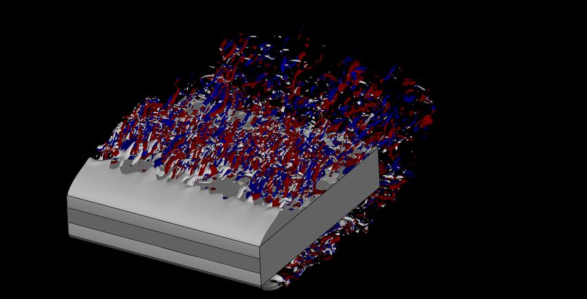
geometry, the flow around a rectangular cylinder contains a rich physics with several
coexisting phenomena: a corner-induced separation, a detached boundary layer that
may become unstable and reattach downstream, several recirculating regions and a
large wake. Depending on the aspect ratio A = L/D (where L and D are the longi-
tudinal and vertical sizes of the body), the rectangular cylinder spans the overall range
of blunt bodies from a flat plate normal to the flow (A → 0), to a square cylinder
(A = 1) and to a flat plate parallel to the flow (A → ∞). At low values of the
Reynolds number Re and for A ≥ 3, leading-edge (LE) and trailing-edge (TE) vortex
shedding are interlocked to a unique frequency as a result of the interaction between
the impinging shear layer instability and the TE shedding [14, 15, 26, 27]. When A
is increased, the Strouhal number based on L and the incoming velocity faces an (al-
most) stepwise increase, depending on the number of vortices shed by the LE shear
layer that are simultaneously present over the cylinder side; see [31, 30, 32, 40]. At
higher Re, the picture complicates even further, with large-scale vortices coexisting
and interacting with small-scale turbulent fluctuations.
     The value A = 5 defines the international benchmark known as BARC (Bench-
mark of the Aerodynamics of a Rectangular 5:1 Cylinder) [3]. The goal of the BARC
is to develop best practices for both experiments and simulations and to qualitatively
and quantitatively characterise the main features of the flow, such as the shedding fre-
quency and the main recirculating regions of the mean flow. An overview of the con-
tributions to the BARC benchmark is provided in [5] and in the more recent works by
[34, 24, 25, 23, 36, 29]. Bruno et al. in [5] pointed out that, despite the fixed value
of A, a significant variability of the available data remains, that complicates the flow
characterisation. This is due to the strong sensitivity of the flow to several aspects of
both experiments and numerical simulations (mainly RANS and LES studies). For the
experiments, critical issues are e.g. measurements uncertainties, geometrical imper-
fections of the model, free stream turbulence. For numerical simulations, instead, we
mention RANS and LES turbulence modelling, various discretisation choices and the
numerical method itself. In a scenario of highly scattered data, [13] performed the first
Direct Numerical Simulation (DNS) of the BARC flow in turbulent regime employ-
ing the finite-volume toolbox OpenFOAM [41], at relatively low Reynolds number
Re = 3000. Our own contribution [8] consisted in replicating that work by using an
in-house finite-difference code and a finer grid to assess the robustness of the available
results.
     BARC data from numerical simulations tend to deviate significantly from those
obtained with experimental measurements. For example, [5] report that the recircu-
lation region over the cylinder side differs, with highly-resolved LES simulations not
matching experiments with their prediction of a consistently shorter recirculation. Be-
sides turbulence modelling, numerical discretisation and experimental uncertainties,
such discrepancies may derive from differences in the setup, i.e. the boundary condi-
tions at the inlet and spanwise boundaries and the inherent geometrical imperfections
of the experimental models. In the numerical simulations the inlet condition is that of
an unperturbed flow parallel to the rectangular cylinder without free-stream turbulence,
but in experiments the incoming flow is less deterministic than that. This aspect was
already found by Mannini et al. [23] to affect the longitudinal extent of the main recir-
culating region. They studied experimentally the effect of free-stream turbulence and

                                            2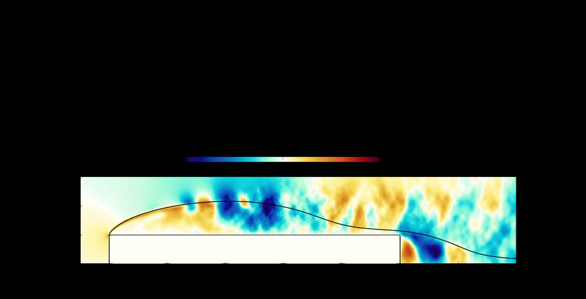
of the angle of attack on the main features of the BARC flow, finding that an increase
of the free-stream turbulence shifts upstream the peak of the root-mean-square value
of the pressure coefficient, implying a decrease of the length of the main recirculat-
ing region over the cylinder [17]. In the spanwise direction, almost every numerical
simulation employs periodic boundary conditions, which are clearly different from a
wind-tunnel experiment where a solid wall exists. However, Bruno et al. [4] have
shown that this boundary condition does not significantly affect the size of the main
recirculating bubble.
    The present work focuses on the geometrical representation of the corners. Per-
fectly sharp corners are obviously just an idealisation: a laboratory model will always
have corners affected to some extent by manufacturing inaccuracies. The effect of
rounding the corners has been mostly studied for a square cylinder (where the re-
circulation region on the side is missing) by for example [33] and [7] for low and
high Reynolds numbers. For rectangular cylinders with larger A we recall the works
[18, 19] that investigate both three-dimensional and two-dimensional infinite D-shaped
bodies changing the curvature radius R of the upstream corners. [10] investigated the
effects of different geometrical peculiarities such as the LE corners and the presence
of a TE on the main flow features. [9] studied how rounded LE and TE corners affect
the occurrence of the first instability. Recently, [37] used an implicit LES to carry out
a sensitivity analysis of the BARC flow to the rounding of the LE corners. They identi-
fied the inadequate treatment of the corners as one of the reasons for the disagreement
between numerical and experimental data. Indeed, they found that introducing even
a tiny curvature radius is enough to significantly enlarge the size of the main recircu-
lating region, thus reducing the discrepancy with the experimental data. However, the
generality of this result with respect to both the Reynolds number and the numerical
approach remains to be ascertained, and this is one of the two goals of the present
contribution.
    The other goal is addressing the accuracy losses induced in a numerical simulation
of the BARC flow by the presence of a perfectly sharp corner. An ideal geometry can be
easily achieved in a numerical simulation, but the geometrical singularity of the corner
leads to a mathematical singularity for the Navier–Stokes equations, with extremely
large velocity derivatives. As a result, the computational grid must be extremely fine
near the corner to avoid a local accuracy drop. As an example, in [8] the DNS by [13]
was repeated with a finer grid and the fluctuations of the lift coefficient were found
to be much larger, because the finer grid captures better the flow separation. This is
also supported by the laminar results of [39] and [1]. Unfortunately, the requirement
of a very fine grid becomes more difficult to satisfy as Re is increased, and renders
DNS simulations at the large Reynolds numbers typical of the experiments extremely
expensive if not impossible. There are however workarounds to cope with the corner
singularity, so that the local solution accuracy can be maintained without resorting to
excessively fine grids; see for example [2]. Among them we recall those based on
the concept, first described by Moffat in [28], that in the vicinity of the corners the
flow is well described by the Stokes equations, which can be dealt with analytically.
Previous examples where the Stokes solution was successfully used to improve the
Navier–Stokes solution near corners include classic fluid dynamics problems such as
the square cavity, see for example [20].

                                           3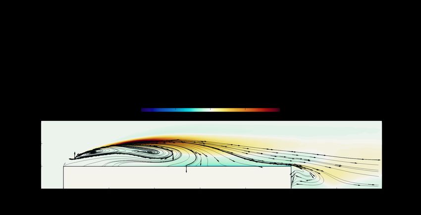
42D

                                                                D

                                                       L = 5D

                                                                42.5D
U∞
          y        5D
                                                 20D
               x
              z

Figure 1: Sketch of the computational domain for the BARC flow, with the reference
system.

     This work consists in a DNS study of the turbulent BARC flow where the focus
is on the LE corners. In a first part, the work [37] is reconsidered with DNS, and
the effect of rounded LE corners is studied by considering two small curvature radii,
i.e. R/D = 1/128 and R/D = 1/64. Compared to the reference work, we use a
higher-fidelity numerical approach without modelling error, but at the cost of a lower
Reynolds number, which is set to Re = 3000 as in our previous DNS [8] used here
as baseline. In a second part, the corners are considered to be sharp, but we employ
the method described in [20] for corner correction, applied to the BARC flow for the
first time. The method is presented in a form tailored to the BARC geometry, and the
changes on the main features of the flow are discussed.

2    The computational approach
Figure 1 shows the geometry, the reference system and the notation. A Cartesian ref-
erence system is used with the origin placed at the LE of the cylinder. The cylinder
has length L and thickness D, curvature radius R of its LE corners, and it is immersed
in a uniform stream with velocity U∞ aligned with the x direction. The y and z axes
indicate the vertical and spanwise directions, respectively. The Reynolds number is
based on the incoming velocity, the cylinder thickness and the kinematic viscosity ν
and is set to Re ≡ U∞ D/ν = 3000 for all the considered cases.

                                          4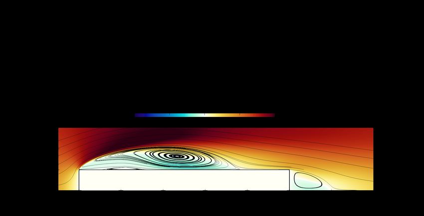
The flow is governed by the incompressible Navier–Stokes equations:

                          ∂u                     1 2
                             + (u · ∇) u = −∇p +    ∇ u
                          ∂t                     Re                                   (1)
                          ∇·u=0

where u = (u, v, w) is the velocity vector and p is the pressure. All quantities are
made dimensionless with U∞ and D. The mean field is indicated with capital letters,
i.e. U = (U, V, 0) and P , while the fluctuations are indicated with a prime, u0 =
(u0 , v 0 , w0 ) and p0 . The computational domain extends from −20 ≤ x ≤ 42.5, −21 ≤
y ≤ 21 and −2.5 ≤ z ≤ 2.5, with the cylinder placed at 0 ≤ x ≤ 5, −0.5 ≤ y ≤ 0.5
and −2.5 ≤ z ≤ 2.5. No-slip and no-penetration conditions are imposed at the cylinder
surface, the unperturbed velocity u = (U∞ , 0, 0) is assigned at the inlet and at the
far field; periodic conditions are used at the spanwise boundaries to account for the
spanwise homogeneity and a convective outlet condition ∂u/∂t = U∞ ∂u/∂x is set at
the outlet boundary.
     The Navier–Stokes equations are solved using the DNS code introduced by [22] and
already used for the BARC flow simulation in [8]. It solves the governing equations
in primitive variables and employs second-order finite differences on a staggered grid.
The cylinder is represented via an implicit, second-order accurate immersed-boundary
method introduced in [21]. For further details on the numerical method see [8], from
which also the discretisation choices are derived. The number of points is Nx = 1776,
Ny = 942 and Nz = 150 in the three directions. An uniform distribution is employed
in the spanwise direction, whereas a geometric progression is used for the streamwise
and vertical directions to properly refine the flow region close to the LE and TE corners,
where the spacing is ∆x = ∆y ≈ 0.0015.
     The present work describes the results of three new simulations carried out on pur-
pose and compares them to the baseline results taken from [8]. Two cases are for the
rounded LE corners and the third case deals with the analytical corner correction. The
rounding is quantitatively defined by the radius R of the inscribed quarter circle. Two
curvature radii have been considered, namely R/D = 1/128 and R/D = 1/64, and
denoted in the paper as cases C1 and C2. The number of points spanning the curvature
radius are 6−7 for case C1 and twice that for C2. The simulations are advanced in time
using a varying time step to ensure that the Courant-Frederic-Levy CFL number re-
mains at CF L ≤ 1, corresponding to an average value of the time step of ∆t ≈ 0.0013.
Before collecting statistics, every simulation is advanced in time long enough to reach
a statistically-stationary state. For the simulations with rounded LE corners, statistics
are collected over 300D/U∞ time units and 300 flow fields are sampled at unitary time
separation. For the simulation with the analytical corner correction, statistics are col-
lected for a total time of 470D/U∞ , again with a unitary sampling time. To increase
the statistical sample, symmetries of the flow in the vertical direction are used. Thus,
mean quantities, indicated by the operator h·i, are computed by averaging in time and
exploiting both the homogeneity in the spanwise direction and the statistical symmetry
in the vertical direction.

                                            5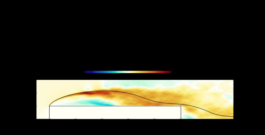
Figure 2: Mean flow. Top: streamlines and color contour for the mean streamwise
velocity component U . Bottom: mean pressure P .

                                      6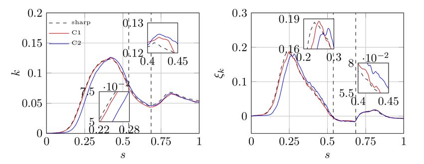
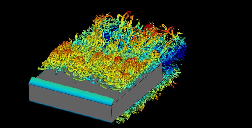
Figure 3: Vortical structures in an instantaneous snapshot. Left: isosurface λ2 = −10
coloured with |y|; the blue-to-red colourmap goes from |y| = 0.5 to |y| = 1.75. Right:
isosurfaces of ωx = 10 (red), ωx = −10 (blue) and |ωz | = 17 (grey).

2.1   The mean and instantaneous flow
To set the stage, the mean flow obtained with the reference sharp LE corners is briefly
illustrated. For further details see [8]. Figure 2 plots the mean streamlines superim-
posed on the map of U in the top panel and the mean pressure P in the bottom panel.
A shear layer with negative vorticity starts from the sharp LE corner; the flow reat-
taches over the cylinder side before eventually separating again at the TE. Three areas
of recirculation can be identified: two of them are above the longitudinal side of the
cylinder and one is in the wake region. The first recirculating region is delimited by
the shear layer separating at the LE and reattaching at xr ≈ 3.955, and it is hereafter
referred to as the primary vortex. Its centre of rotation, i.e. the elliptical stagnation
point with U = V = 0, is placed at (x, y) ≈ (2.357, 0.83). As shown in the bottom
panel, the core of the primary vortex shows large negative values of pressure. Within
the primary vortex, a smaller counter-rotating recirculating region is present, hereafter
referred to as the secondary vortex. It is generated by the reverse boundary layer in the
near-wall region of the primary vortex, which separates moving upstream owing to the
adverse pressure gradient [38]. The secondary vortex extends for 0.63 ≤ x ≤ 1.59
and its centre of rotation is placed at (x, y) ≈ (1.2, 0.541). The third recirculating
region in the wake, hereafter referred to as wake vortex, is delimited by the shear layer
separating from the sharp TE. Its centre of rotation is placed at (x, y) ≈ (5.415, 0.25)
and extends up to x ≈ 5.947.
    Figure 3 shows the turbulent structures populating an instantaneous snapshot of the
BARC flow. They are visualised as isosurfaces of the second larger eigenvalue λ2 of
the velocity gradient tensor [16]. Contours of streamwise and spanwise vorticity ωx
and ωz are also used to visualise the orientation of the structures.
    After the LE separation, the flow remains initially laminar, until at x ≈ 0.5 a
Kelvin–Helmholtz instability of the shear layer occurs, which breaks it into large-scale
spanwise tubes. Moving downstream the tubes are stretched by the mean gradient and
roll up, originating hairpin-like structures. Further downstream a complete transition
to turbulence is observed. The hairpin vortices break down into elongated streamwise

                                           7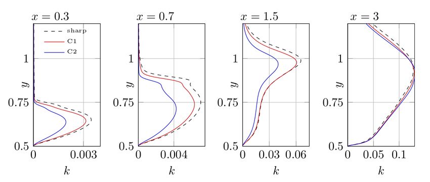
Table 1: Comparison of size and positions of the three recirculating regions, for the
cases with rounded corners and the reference one with sharp corners from Ref. [8].
xs and xe are the start and end coordinates, and L indicates the length of each region,
whereas xc and yc are the coordinates of their centre of rotation.
                                        sharp             C1              C2
                           xs,1            0            0.005             0.01
                           xe,1         3.955           3.895             3.89
     Primary vortex
                            L1          3.955            3.89             3.88
                         (xc , yc ) (2.357, 0.83) (2.361, 0.81)      (2.43, 0.81)
                           xs,2          0.63            0.75             0.97
                           xe,2          1.59           1.585             1.75
    Secondary vortex
                            L2           0.96           0.835             0.78
                         (xc , yc ) (1.2, 0.541) (1.17, 0.531) (1.315, 0.533)
                           xs,3            5               5                5
                           xe,3         5.975            6.01             6.02
      Wake vortex
                            L3          0.975            1.01             1.02
                         (xc , yc ) (5.415, 0.25) (5.425, 0.25        (5.43, 0.25)

vortices that are easily visualised by the positive and negative contours of ωx . In this
region of the flow the large-scale motions derived from the Kelvin–Helmholtz insta-
bility coexist with the small-scales structures associated with the turbulent motions.
Finally, at the TE the flow separates again and the turbulent structures are convected in
the turbulent wake.

3     Rounding the LE corners
This section discusses the effects of rounding the LE corners. Two rather small cur-
vature radii characterize cases C1 and C2, since the aim of the present work is to
investigate the effect of manufacturing imperfections on the BARC flow.

3.1    The mean flow
The mean flow with rounded corners closely resembles the one of the reference con-
figuration with sharp corners [8], with only small changes in the size of the three re-
circulating regions and in the position of their centre of rotation. These changes are
summarised in table 1, where the extent of the three recirculating regions and the posi-
tion of their centre of rotation are reported.
    How rounding affects the primary and wake vortices is shown by the streamline
passing near the sharp LE, shown in figure 4. The starting point of the streamlines is
placed just above the LE corner at (x, y) = (0, 0.5001) for both the sharp and rounded
configurations, although in the latter cases the actual separating point is slightly shifted
downstream; see table 1. The differences shown in figure 4 have been verified to be
robust to small shifts of the seeding point. This streamline delimits first the primary
vortex and then, after passing over the trailing edge, the wake vortex. Close to the

                                             8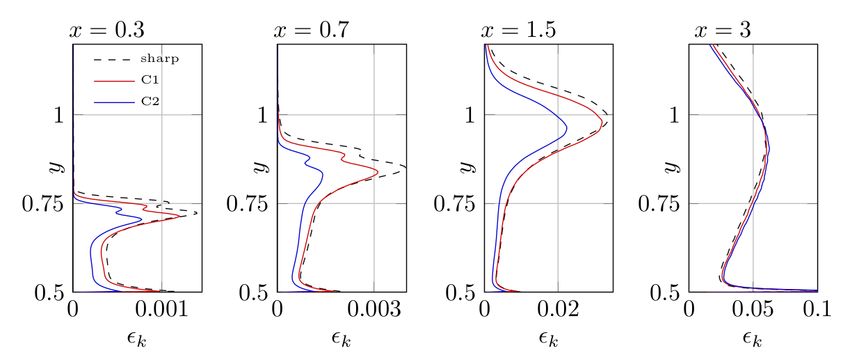
1.5
                         sharp
                         C1                    1.08
                         C2                    1.05
              1                                                      0.54
                                                  1.75    2   2.25
                                                                     0.52
                       0.56                                           0.5
         y
                                                                        5.25 5.35 5.45
             0.5
                        0.5
                              0   0.04

                   0                     2.5                    5                   7.5
                                                      x

Figure 4: Mean streamline passing through the point (x, y) = (0, 0.5001), for the sharp
and rounded configurations. The zoomed insets highlight three regions close to the LE,
close to the top of the primary recirculation, and in the near wake.

Figure 5: Vertical profiles of the streamwise component of the mean velocity U at four
different stations over the cylinder side.

separation point the line has a lower slope in the rounded cases, indicating a lower
inclination of the shear layer. At x ≈ 2 the streamline shows that the vertical extent of
the primary vortex decreases for increasing values of R. Finally, when the streamline
crosses the TE a milder slope develops, consistently with the smaller extension of the
wake vortex reported in table 1.
    Figure 5 presents the vertical profile of the U velocity component at different
streamwise locations over the cylinder side, i.e. x = 0.3, 1.1, 2, 4.5. The first three
panels describe the changes within the primary vortex. As shown in figure 4, the
rounded corners lead to a slightly reduced vertical extent of the primary vortex, as
the shear layer separates from the LE with a lower angle. This is also conveniently
visualised by the coordinate yU =0 where the mean streamwise velocity component be-
comes zero. In the first portion of the primary vortex yU =0 is shifted towards the wall
in the rounded configurations; see the two left panels of figure 5. Moving downstream
for x ≥ 1.5, instead, the difference is less evident indicating that the main changes are

                                                  9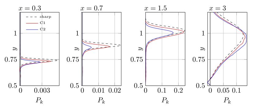
localised close to the LE; see the third panel where yU =0 is almost the same for the
sharp and rounded configurations. A decrease of the shear-layer separation angle is
consistent with a lower longitudinal size of the primary vortex, which is seen in table
1 to decrease from L1 = 3.95 to L1 = 3.89 for case C1 and L1 = 3.88 for C2, i.e.
approximately 2%. A further effect of the rounding is the decrease of the backflow in
the core of the primary vortex shown at x = 2, where U is less negative in the rounded
configurations. This is consistent with the results of [19] who analysed the effect of
(large) LE roundings on infinite D-shaped bodies. Interestingly, the rounded corners
also affect the mean field after the reattachment, as seen in the last panel of figure
5 at x = 4.5, where the mean flow is accelerated. This is explained by the slightly
lower extension of the primary vortex that enables a larger development of the succes-
sive boundary layer before its separation, and is associated to an enhancement of the
turbulent activity as shown in the following section.
    Table 1 quantifies the modifications of the three main vortices. When the LE cor-
ners are rounded, the upstream separation point slightly moves downstream and is
found close to the end of the curvature, where a second-derivative discontinuity takes
place. we found the primary vortex to start at xs,1 = 0.005 for C1 and at xs,1 = 0.01
for C2. As already mentioned, this small downstream shift together with the decrease
of the shear layer separating angle leads to a decrease of the longitudinal and vertical
extensions of the primary vortex. The same effect has been found in preliminary two-
and three-dimensional simulations (not shown here) in the laminar regime at Re = 500,
with 1/128 ≤ R/D ≤ 1/2. The centre of rotation of the primary vortex slightly moves
towards the reattachment point as R increases, consistently with the results of [19].
Rounding the corners also affects the smaller secondary vortex. Indeed, for both C1
and C2 we have found that its longitudinal size consistently decreases up to L2 ≈ 0.835
(≈ −12%) for C1 and L2 ≈ 0.78 (≈ −18%) for C2. However, in the two rounded
cases there are some differences. For C1 the position of the centre of rotation is almost
unchanged, since xs,2 moves downstream and xe,2 moves upstream. For C2, instead,
the decreased size of the recirculating vortex is accompanied by an overall downstream
shift, as indicated by the positions of xs,2 , xe,2 and of the centre of rotation. Interest-
ingly, the LE rounding also affects the size of the wake vortex. Indeed, by increasing
the curvature radius its length slightly increases up to L3 ≈ 1.01 for C1 (≈ +3.5%)
and up to L3 ≈ 1.02 for C2 (≈ +4.5%). Such modifications are consistent with the
acceleration of the flow in the last part of the cylinder side, resulting in a shear layer
that separates from the sharp TE with larger velocity.

3.2    Turbulent kinetic energy
Rounding the corners also affects the fluctuating velocity field. Figure 6 plots the
turbulent kinetic energy k = hu0i u0i i/2 (repeated index implies summation) for the sharp
configuration; figure 7 plots vertical profiles of k at different streamwise locations, i.e.
x = 0.3, 0.7, 1.5, 3, for the sharp and rounded cases. Close to the LE, i.e. for x < 1,
k is very small, confirming the almost laminar flow state. Moving downstream, k
quickly increases indicating a sharp transition to the turbulent state, as can be seen by
inspecting an instantaneous velocity field in figure 3. The turbulent activity is most
intense in the core of the primary vortex as indicated by the maximum of k found at

                                            10
Figure 6: Map of the turbulent kinetic energy for the sharp configuration.
Figure 7: Vertical profiles of the turbulent kinetic energy k at four different stations
over the cylinder side, i.e. x = 0.3, 0.7, 1.5, 3.
11(x, y) ≈ (2.7, 0.96); however large values of k are observed also in the near-wake
region close to the TE as shown by the presence of an additional local peak at (x, y) ≈
(6.15, 0.36).
For C1 the vertical profiles of k are very close to those of the sharp configuration.
This further confirms that – at least at this Reynolds number – a small rounding of the
LE corners does not lead to an abrupt change of the flow topology. In the rounded con-
figuration the intensity of the velocity fluctuations decreases only near the LE: it seems
that the rounded corners lead to a spatial delay of the development of the velocity fluc-
tuations, in agreement with the results of [37, 18, 19, 10]. Close to the LE, the profiles
of k show a well-defined peak in correspondence of the shear layer (see the first three
panels of figure 7). This agrees with the notion that, close to the LE, the fluctuations
are mainly generated by the Kelvin-Helmholtz instability of the shear layer. Moving
downstream, k becomes distributed over a wider range of y, until a completely turbu-
lent state is reached and large values of k are observed in the overall extension of the
primary vortex, revealing the presence of other production mechanisms. Interestingly,
for x ≥ 2.5 the intensity of k for y ≤ 1 is larger in the rounded configurations, consis-
tently with the picture of a delayed development of the turbulent fluctuations; see the
right panel of figure 7. This accompanies the increased U observed in this region of
the flow. Moreover, in the rounded cases, owing to the reduced vertical extent of the
primary vortex, k drops to almost zero at lower y compared to the sharp configuration.
The delay in the development of the turbulent kinetic energy in the rounded con-
figurations and the larger k observed after the reattachment point, may be explained by
the differences in the production Pk and dissipation k in its budget. These terms read
0 0 ∂U 0 0 ∂V 0 0 ∂U ∂V
Pk = −hu u i −hv v i −hu v i + , (2)
∂x ∂y ∂y ∂x
0
∂u ∂u0
0
∂v ∂v 0
0
∂w ∂w0
k = ν +ν +ν , (3)
∂xj ∂xj ∂xj ∂xj ∂xj ∂xj
where repeated indices imply summation.
Figure 8 plots the map of the production for the reference sharp configuration; fig-
ure 9, instead, plots vertical profiles of Pk at different streamwise positions over the
cylinder side, i.e. x = 0.3, 0.7, 1.5, 3, for the sharp and rounded configurations. For
x ≤ 0.5 low values of Pk are observed, which is consistent with the low values of k
in figure 6. Along the shear layer Pk is positive, but it becomes negative just below.
However, as already discussed in [8], this negative Pk does not correspond to the nega-
tive production rate of k localised in the shear layer seen by [12]. Moving downstream
at x ≈ 1.3, Pk peaks in correspondence of the shear layer. This implies that, when
the Kelvin–Helmholtz instability takes place, energy is being drained from the mean
flow to feed the fluctuating field. Further downstream, large values are observed also
at lower y in the core of the primary vortex indicating that a further production mech-
anism different from the Kelvin–Helmholtz instability of the shear layer is occurring.
Arguably, this is associated to the interaction between the streamwise-aligned vortices
observed in figure 3 to populate this region of the flow and the large mean velocity
gradients. For x ≥ 2.5 a region with slightly negative Pk is observed in the vicinity of
the cylinder side, indicating that energy feeds back from the fluctuations to the mean
12Figure 8: Map of the production term Pk of the turbulent kinetic energy for the sharp
configuration.
Figure 9: Vertical profiles of Pk at four different station over the cylinder side as in
figure 7.
13Figure 10: Map of the dissipation rate of the turbulent kinetic energy
field. Thus, despite the presence of the wall, the mechanism sustaining the turbulent
fluctuations close to the longitudinal side of the cylinder differs from what observed in
the canonical wall-bounded flows, where Pk is always positive. Finally large positive
values of Pk are found in correspondence of the shear layer separating from the TE,
again due to the larger mean velocity gradients.
Figure 9 show that, close to the LE, the production decreases when the corners are
rounded. More downstream, as already observed for k, the differences between the
three cases shrink, indicating that the production of fluctuating energy in the rounded
cases becomes close to what observed in the sharp configuration. Rounding the LE
corners thus leads to a downstream shift of the Kelvin–Helmholtz shear layer insta-
bility and to a delayed streamwise development of the velocity fluctuations. As also
observed in [19], this may explain the downstream shift of the centre of rotation of
the primary vortex. Indeed, the shift of the instability source turns into an extended
low-velocity region in the upstream part of the primary vortex that is arguably respon-
sible of the downstream shift of the stagnation point. We note again how for increasing
curvature radius the wall distance at which Pk drops to zero becomes smaller, owing to
the decreasing vertical extent of the primary vortex. Interestingly, for x ≥ 2.5 the pro-
duction term of the rounded cases overcomes that of the sharp configuration for y ≤ 1,
indicating that in the second part of the longitudinal cylinder side the production of the
fluctuating energy is enhanced by the rounded corners. This agrees with the slight in-
crease of k in the same region and with the picture of a stronger shear layer separating
from the TE.
Figures 10 and 11 describe the dissipation k . Figure 10 plots the map of k for the
sharp configuration, while figure 11 plots vertical profiles of k for the three considered
cases at four different streamwise locations, i.e. x = 0.3, 0.7, 1.5, 3. Large values of
k occur in the shear layer for x ≥ 1, in the core of the primary vortex and close to the
cylinder side for x ≥ 2.5, where viscous effects dominante. For x < 1, instead, the
values of k are much lower as the turbulence activity is locally scarce compared to the
rest of the domain. As for production, the main differences between the rounded and
sharp configurations are observed for x < 2.5 where rounding leads to a decrease of
k in the overall extent of the primary vortex, in agreement with a picture of lower tur-
14Figure 11: Vertical profiles of the dissipation rate of the turbulent kinetic energy at four
different stations over the cylinder side.
bulent activity. Moving downstream, instead, the differences among the three profiles
strongly decrease until for x ≥ 2.5 k becomes slightly larger in the rounded config-
urations for y ≤ 1. Note however that here the increase of Pk in the rounded cases
is larger than the increase of k . Therefore, this results in a net increase of the source
term ξk = Pk − k that determines an intensification of the spatial transports of k.
Although there is no direct link, this may explain at least partially the larger values of
k observed in figure 7 for the rounded cases. The spatial transport of k is visualised by
the two-dimensional flux vector ψ defined as [35]:
1 0 0 0 1 ν ∂
ψj = ui ui uj + p0 u0j + Uj hu0i u0i i− hu0i u0i i with j = x, y (4)
2
| {z } | {z } | {z } |2 ∂x{z
2 j
turbulent transport pressure transport mean transport
}
viscous diffusion
where repeated indices imply summation. Note that this is half of the sum of the
flux vector for the three normal stresses discussed in [8]. Figure 12 plots the field
lines of the flux vector over the colour contour of the source term ξk , or equivalently
∇ · ψ. The fluxes allow a precise description of the spatial transfer, and their field lines
visualise how the kinetic energy is transferred in space. Therefore, the fluxes explain
the different positions at which k and ξk have their peak. Their divergence, ∇ · ψ,
provides quantitative information about the energetic relevance of the fluxes. When
∇ · ψ is positive, i.e. ξk > 0, the fluxes are energised by local production mechanism.
In contrast, when ∇ · ψ is negative the fluxes release energy to sustain locally the
fluctuations. The flux lines originate where ∇ · ψ has large positive values and vanish
where ∇ · ψ is negative.
The large contribution of the Kelvin–Helmholtz instability to Pk yields large ξk >
0 along the shear layer with a peak at (x, y) ≈ (1.7, 1); as expected the largest values
are slightly shifted downstream in the rounded cases. Close to the cylinder side, i.e.
approximately for y ≤ 0.75, the negative contribution of k dominates and leads to
ξk < 0. A further region of positive ξk is observed in correspondence of the TE
shear layer. The fluxes of k differ from the fluxes of the three normal stresses. The
large values of ξk in correspondence of the shear layer energise all the fluxes that in
15Figure 12: Field lines of the flux vector ψ and colormap of the source ξk = Pk − k
for the reference sharp configuration. The arrows are tangent to the flux vector ψ and
provide directional information.
turn transfer the excess of k over the entire domain. Four different types of lines are
observed, which relate to different transport mechanisms. Some lines pass over the
TE at relatively large y and, dominated by the mean transport, continue in the wake
region. A second group of lines passes very close to the TE and then they are further
energised by the positive ξk in the separating shear layer. These lines then vanish in
correspondence of the rear vertical side of the cylinder, after having released k within
the wake vortex. These two groups of field lines indicate that the flow over the cylinder
side influences both the wake vortex and the downstream wake.
The other two types of lines remain confined within the primary vortex, point-
ing to a self-sustaining mechanism, as predicted by [11]. Some are attracted by the
cylinder side in the whole range 0 ≤ x ≤ 5, indicating that part of the excess of
k produced by the Kelvin–Helmholtz instability is released near the wall where it is
partially dissipated by viscous effects and partially feeds the mean flow (recall the
negative values of Pk ). The last type of lines shows a spiral-like behaviour in the up-
stream part of the cylinder side. Such lines indicate that part of the k produced by
the Kelvin–Helmholtz instability is transported and released upstream to feed the flow
region close to the LE. This spiral-like pattern has two singularity points the lines are
attracted to. For the sharp configuration they are located at (x, y) ≈ (0.6, 0.81) and
(x, y) ≈ (1.8, 0.85). For the rounded configuration C1 the qualitative differences on
these transfers are small, confirming again that a small rounding does not lead to an
abrupt change in the transport of k. However, for C2 differences are more significant.
In particular, the spiralling pattern is shifted downstream: the upstream singularity
point moves to (x, y) ≈ (0.87, 0.83). Overall, this means that in the rounded configu-
rations the downstream shift of the Kelvin–Helmholtz instability is accompanied by a
downstream shift of the transfer mechanism involving the upstream part of the primary
vortex. Therefore, both effects are responsible of the decrease of the intensity of k in
the region close to the LE.
Changes of k, Pk and k can be summarised by tracking them along the streamline
starting just above the upstream separating point shown in figure 4. This is visualised
16Figure 13: Evolution of k (left) and ξk (right) over the mean streamline originating at
(x, y) = (0, 0.5) shown in figure 4 as a function of the normalised curvilinear coordi-
nate s. The left vertical dashed line marks the reattachment point, and the right dashed
line marks the TE.
in figure 13 where both k and ξk are plotted as a function of the curvilinear coordinate
s normalised with the length ` of the streamline:
1 `
Z p
s= ds with ds = dx2 + dy 2 ;
` 0
For s ≤ 0.15 both ξk and k are almost null, indicating the negligible turbulent activity
in the first portion of the separating shear layer. For larger s ξk and k show an abrupt
increase due to the occurrence of the Kelvin–Helmholtz instability. The largest values
of k are slightly delayed compared to the largest values of ξk due to the action of the
mean convection. Then, at larger s, both k and ξk decrease again. In the rounded
cases these variations are shifted towards larger s, consistently with the picture of a
delayed turbulent activity. This results in a lower intensity of both k and ξk before
their maxima, but also in larger intensities at larger s. After the reattachment point
ξk features negative values and becomes a sink for k. Consistently, k decreases in
this region and reaches its minimum in correspondence of the TE. Then, when the
streamline passes over the TE, positive ξk are observed again in correspondence of the
shear layer, while negative ξk are observed downstream, where there is no production
of turbulent fluctuations. This results first in an increase of k, followed by a further
decrease.
3.3 Discussion
The present results provide a picture of curvature-related effects that is not entirely in
agreement with that emerging from the similar study by Rocchio et al. [37]. Indeed, the
two studies possess significant differences, with the latter being based on implicit LES
at the much higher Re = 40000. The range of curvature radii considered in [37] is quite
wide, spanning from R/D = 1/20 to R/D = 1/270, but this should be considered
in view of their significantly higher Re. With this premise, perhaps the main finding
of [37] is that even a tiny curvature radius produces an abrupt change of the mean
17flow, and a sudden enlargement of the primary vortex. On the contrary, our results
indicate that a small amount of rounding does not affect the flow significantly, and that
curvature effects manifest themselves gradually when the curvature radius increases.
Moreover, we have found that the rounding affects the extension of the primary vortex
in the opposite way, as in our experiments its size diminishes. In terms of turbulent
kinetic energy distribution, though, there is qualitative agreement between [37] and the
present results, with differences in the amount of rounding-induced changes that may
simply be due to the different Re.
Assessing the reason(s) for these differences certainly requires further studies. How-
ever, some hypotheses can be put forward. As observed by [19] rounding the LE cor-
ners has two opposite effects. The downstream shift of the Kelvin–Helmholtz instabil-
ity tends to increase the length of the primary vortex, while the decrease of the sepa-
ration angle at the LE tends to decrease it. In the present DNS the latter effect seems
to prevail, while in [37] the former one seems to dominate. Moreover, Ref. [37] inter-
estingly describes the appearance of a region with larger k near the LE not only over
the separated shear layer, but also over the front face of the body, before the separation
point. To explain this observation, that cannot be attributed to an upstream shift of the
shear layer instability, the authors of Ref. [37] mention that the sharp corner might
introduce a large amount of k which is not fully damped in their implicit LES simu-
lation. This suggests the possibility that, at least partially, the large sensitivity to the
curvature radius reported in Ref. [37] is associated to the specific numerical approach.
Indeed, the proper description of a sharp corner, especially at high Re, requires ex-
tremely fine grids, which is the very motivation for our accounting of the geometrical
singularity analytically (see next Sec. 4). A further partial explanation of the discrep-
ancy resides in the different numerical noise produced by the numerical methods used
here and in [37], coupled with the large receptivity of this flow to inflow perturbations.
Indeed, it is well known that numerical errors and interaction between inlet and out-
let boundary conditions can be artificial sources of inflow perturbations, whose level
depends on the accuracy of the numerical method. The receptivity of this flow on the
inflow perturbations has been largely studied to address the discrepancy between nu-
merical simulations and experiments. For example [36] via LES simulations found that
a higher level of incoming turbulence corresponds to a shorter primary vortex and to
an upstream shift of the secondary vortex. [19] observed that this receptivity increases
with the curvatures radius and report that for R/D = 1/2 the size of the primary vortex
decreases of approximately 60% compared to the case without perturbations.
Per se, the present results are self-consistent, and compare well with other similar
numerical analyses of low-Re flow around bluff bodies with rounded LE. For example,
[18] studied a three-dimensional D-shaped body with rounded LE at Re = 2500, and
considered two relatively large curvature radii, i.e. R/D = 1/2.5 and R/D = 1/5. In
qualitative agreement with our results, they observed that increasing R leads to a de-
crease of both longitudinal and vertical extensions of the main recirculating region over
the longitudinal body side. [19] performed two-dimensional and three-dimensional
DNS of the flow past a flat plate with rounded leading edge at Re = 4000, with curva-
ture radius ranging between R/D = 1/2 and R/D = 1/16. Their three-dimensional
simulations confirm that for larger R the extension of the primary vortex decreases.
Moreover, a slight downstream shift of the secondary vortex is observed, which is in
18P
θ
r
y
x
Figure 14: Sketch of the polar coordinate system (r, θ) used to derive the analytical
solution in the neighbourhood of the top LE corner.
line with our results for the R/D = 1/64 case, together with a decrease of the slope
of the separating shear layer. They also find a decrease of the backflow in the re-
gion close to the plate side, in agreement with our simulations. Their two-dimensional
simulations, instead, show completely different results, but it is known that at their
high Re the flow is strongly unstable to three-dimensional perturbations. In contrast,
we have conducted preliminary two-dimensional simulations in the laminar regime
at Re = 500, and these confirm our results in the turbulent regime and agree with
the three-dimensional simulations at the same Reynolds number. This is because at
Re = 500 the three-dimensionality of the flow almost does not affect the mean flow.
Indeed, we have observed that the Re = 500 only slightly exceeds the critical Reynolds
number for the first onset of the first three-dimensional instability. Finally, [10] per-
form LES simulations of a flat plate at Re ≈ 3000 with both sharp and rounded LE
with R/D = 1/2. Again, their results qualitatively confirm that in the rounded config-
uration the extension of the main recirculating region decreases.
4 Corner correction
The two upstream LE corners where the flow impinges before separating are nominally
sharp, and as such constitute a geometrical singularity that locally impacts the solution
accuracy, to an extent that depends on the local fineness of the adopted grid. To over-
come this, one may analytically determine the solution near the corner. In this work we
follow an idea originally introduced by Luchini [20] and later taken up and expanded
in [6]. The strategy leverages the fact that, close enough to the corners, viscous effects
dominate as the velocity gradients become infinitely large. As a result, locally the in-
plane velocity components (i.e. u and v) can be deduced from the Stokes equations,
where the non-linear convective terms of the Navier–Stokes equations are discarded.
4.1 Formulation
One begins by solving the Stokes equation within the portion of plane identified by
two semi-infinite and perpendicular straight lines. In the following discussion we only
describe the case of the top LE corner, shown in figure 14, but the same procedure holds
with obvious modifications for the bottom LE corner. The two-dimensional Stokes
equation is written in a longitudinal, z = const plane in terms of vorticity ω and
19streamfunction ψ, with a polar coordinate system (r, θ) such that x = r cos(θ) and
y = r sin(θ). The equations read:
∂ 2 ψ 1 ∂ψ 1 ∂2ψ
+ + = −ω
∂r2 r ∂r r2 ∂θ2 (5)
∂ 2 ω 1 ∂ω 1 ∂2ω
2
+ + 2 2 =0
∂r r ∂r r ∂θ
where the radial and azimuthal velocity components, ur and uθ are related to ψ by:
1 ∂ψ ∂ψ
ur = , uθ = − . (6)
r ∂θ ∂r
We look for separable solutions in the form:
ψ(r, θ) = P (r)F (θ) ω(r, θ) = R(r)G(θ). (7)
By introducing the functional form above into (5), and requiring the solutions to be
regular when the corner is approached i.e. r → 0, one obtains
P (r) = r(K+2) ; R(r) = rK (8)
and the Stokes problem reduces to the following pair of ODEs:
G00 (θ) + K 2 G(θ) = 0 F 00 (θ) + (K + 2)2 F (θ) = G(θ). (9)
The boundary conditions require the velocity to be zero on the two straight sides of the
corner; in polar coordinates, this translates into:
∂ψ ∂ψ 3π 3π
(r, 0) = 0; ψ(r, 0) = 0; (r, ) = 0; ψ(r, ) = 0. (10)
∂θ ∂θ 2 2
Solving the two ODEs (9) leads to:
G(θ) = A1 cos (Kθ) + A2 sin (Kθ)
F (θ) = B1 cos ((K + 1)θ) + B2 sin ((K + 2)θ) + B3 cos (Kθ) + B4 sin (Kθ) .
(11)
where A1 , A2 , B1 , B2 , B3 , B4 are constants to be determined via the boundary condi-
tions 10. A linear system is obtained:
M (γ)b = 0
where γ = K + 1, and b is the vector of the unknowns b = (B1 , B2 , B3 , B4 ) needed
to determine ψ and therefore ur and uθ . To solve the system we require that
det (M (γ)) = 0
which leads to the following relation:
2 3π
2
γ − sin γ = 0. (12)
2
20The numerical solution of this equation via bisection yields γ ≈ 0.5444837. Then by
solving the linear system, and by taking B = 1 without loss of generality thanks to the
linearity of the problem, the unknowns b are obtained:
B1 = 1
(γ − 1) cos (γ − 1) 3π 3π
2 − (γ − 1) cos (γ − 1) 2
B2 = = D2 (γ)
(γ − 1) sin (γ + 1) 3π
2 − (γ + 1) sin (γ − 1) 2
3π
(13)
B3 = −1
(γ + 1) cos (γ + 1) 3π 3π
2 − (γ + 1) cos (γ − 1) 2
B4 = = D4 (γ).
(γ − 1) sin (γ + 1) 3π
2 − (γ + 1) sin (γ − 1) 2
3π
Once the asymptotic behaviour of ψ(r, θ) in the vicinity of the corner has been
determined, we get ur (r, θ) and uθ (r, θ) by their definitions (6):
ur (r, θ) = rγ ((γ − 1) sin ((γ − 1)θ) − (γ + 1) sin ((γ + 1)θ)+
(14)
D4 (γ)(γ − 1) cos ((γ − 1)θ) + D2 (γ)(γ + 1) cos ((γ + 1)θ)),
uθ (t, θ) = −(γ + 1)rγ ( cos ((γ + 1)θ) + D2 (γ) sin ((γ + 1)θ) −
(15)
cos ((γ − 1)θ) + D4 (γ) sin ((γ − 1)θ)).
Last, the Cartesian velocity components u and v can be easily retrieved by:
u = ur cos(θ) − uθ sin(θ); v = ur sin(θ) + uθ cos(θ). (16)
Pressure is obtained from the Stokes equation in polar coordinates solved for ∂p/∂r,
i.e.: 2
1 ∂ 2 ur
∂p ∂ ur 1 ∂ur 2 ∂uθ ur
=ν + + − − . (17)
∂r ∂r2 r ∂r r2 ∂θ2 r2 ∂θ r2
An integration in r yields:
p(r, θ) = 4νγrγ−1 (D4 (γ) cos ((γ − 1)θ) − D3 (γ) sin ((γ − 1)θ)) . (18)
Once the correct local behaviour of u, v and p in the vicinity of the corner is an-
alytically determined, this information is used in the DNS code, in such a way that
the DNS solution possesses the required characteristics. The general idea is to use the
exact Stokes solution to enforce a deferred correction of the DNS solution via two cor-
rection terms, one for the momentum equations in the x direction and one for that in the
y direction, that are used at each iteration to ensure that the updated solution satisfies
the Stokes equation in the vicinity of the corner. In the following the region near the
corner interested by the correction is defined by:
(x − xc )2 + (x − yc )2 ≤ (0.1D)2
where (xc , yc ) are the coordinates of the corner. In the present work we choose to
apply the correction within a distance of 0.1D from the corner, that is enough to let the
correction decrease to zero, but it must be noted that the distance needs to be accurately
tuned, to avoid an incomplete correction due to an excessively short distance.
21Figure 15: Effect of the analytical correction of the LE corner singularity on the mean
flow. Top panel is for δU = Uc − Ur while the central one for δV = Vc − Vr ,
where subscripts ·c and ·r refer to the corrected and the reference case. The black line,
drawn for the reference case, indicates the streamline originating from just above the
LE corner and locates the shear layer. The bottom panels show a zoom on the LE
corner for δU (left) and δV (right).
224.2 Results
The improvement made possible by the analytical correction for the LE corner singular-
ity are considered here in terms of mean flow. Since the nominal geometry is the same,
they can be simply expressed in terms of the difference between the two mean fields,
with and without correction. Note that the very fine grid of the reference flow is used,
and this precludes observing potentially large benefits. The goal of the present work is
only the qualitative description of the effects induced by the analytical correction.
Figure 15 plots the difference of the mean velocity field in terms of its two compo-
nents,
δU = Uc − Ur and δV = Vc − Vr ,
where the subscripts ·c and ·r refer to the case with the analytical correction and to
the reference case without it. The following discussion only considers the top side of
the cylinder, but the same observations are valid for the bottom side too, by suitably
accounting for the symmetries of the flow. The black solid line is the streamline of
the reference case starting just above the top LE corner at (x, y) = (0, 0.5001), and
is useful to locate the shear layer. The maps of δU and, to a larger extent, δV both
reveal the presence of a small amount of statistical noise, due to the finite temporal
average. However, the robustness of the observations has been checked by computing
the maps with only half of the sample size; the noise is correspondingly increased, but
the qualitative scenario remains unchanged.
Near the LE corner, where the analytical correction is directly applied, both δU and
δV are positive in the shear layer. On the other hand, just before the corner there are
two tiny regions with δU < 0 and δV < 0 attached to the vertical side of the cylinder.
This indicates that the corrected flow is decelerated just before its impingement on
the corner, whereas the shear layer separating from it is accelerated. The maps of δU
and δV show that in the flow with correction the streamlines more closely follow the
geometry of the corner, as explained in the following discussion. The local slope of a
mean streamline ys (x) is defined as:
dys V
= .
dx U
Therefore the slope change induced by the correction is
dys Vc Vr Ur Vc − Uc Vr
δ = − = .
dx Uc Ur Uc Ur
This quantity is plotted in figure 16, where blue indicates δ(dys /dx) < 0 and orange
δ(dys /dx) > 0. Just before the corner δ(dys /dx) is positive for 0.4 ≤ y ≤ 0.5; note
that this vertical extension almost corresponds to the distance chosen for the correction
to apply. This indicates that the corrected streamlines are more vertical in this region
and therefore more aligned with the vertical side of the cylinder. On the other hand, the
blue region after the corner indicates that the streamlines, after crossing the LE, have a
lower slope and align better to the longitudinal side of the cylinder. In other words, the
separation angle of the shear layer decreases once the analytical correction is used.
The analytical correction acts locally near the corners, but its effects are seen also
further from it, in the entire region above the cylinder side. For example, similarly to
23Figure 16: Sign of the change δ(dys /dx) in the local slope of mean streamlines. Blue:
negative change; orange: positive change.
what previously observed for the rounded configurations, the decrease of the separation
angle of the shear layer results in a slight decrease of both the vertical and longitudinal
extent of the primary vortex, with L1 dropping from 3.955 to 3.92 (≈ −1.3%). The
top panel of figure 15 indicates that within the primary vortex the analytical correction
yields δU > 0 almost everywhere but close to the cylinder side for x ≥ 2.5, where
δU < 0 shows an increase of the backflow. The positive δU > 0 in the region around
the limiting streamline is consistent with a smaller vertical extent of the primary vortex.
On the other hand, after the first portion of the shear layer where δV > 0, for inter-
mediate x δV becomes negative and then positive again after the reattachment point.
This once again agrees with the picture of a shorter primary vortex. Indeed this change
of the sign of δV is due to an upstream shift of the point at which the streamlines turn
towards lower y.
The small differences between the reference case and the case with the analytical
correction confirm that the resolution used in this work near the LE corners is more
than adequate. We expect that increasing the resolution further would lead eventually
to vanishing differences.
5 Conclusions
The present work has studied via Direct Numerical Simulations (DNS) the BARC
benchmark flow in the turbulent regime at Re = 3000, with focus on the geometrical
characterisation of the leading-edge (LE) corners. In doing so we intend to contribute
to the discussion whether the geometrical details of the nominally sharp LE corners
could explain at least partially the scatter of available data.
In the first part of the work, the effect of rounded LE corners has been studied.
Two values for the curvature radius r have been considered, namely R/D = 1/128
and R/D = 64, which mimic the unavoidable imperfections that would be present in a
physical model owing to manufacturing procedures. The present investigation follows
a similar one by [37], who simulated the flow via Large Eddy Simulations at a much
larger Reynolds number, i.e. Re = 40000. We have discussed the possible reasons
24for differences between that study and the present results, which may be traced down
to the significantly different Reynolds number combined with the different modelling
approach and numerical method. Unlike in [37], we have found that a small amount of
rounding does not abruptly change the features of the mean flow, and that the effects
increase gradually with r. In the rounded configurations, the shear layer separates
from the LE with a milder slope, so that the vertical and longitudinal sizes of the main
recirculating region are both reduced. Interestingly, rounding the LE corners has been
found to affect the wake vortex too, with its longitudinal size slightly increasing with
R. This is explained by the observation that rounding the LE increase the velocity over
the last part of the cylinder side after the reattachment point, resulting in a faster TE
shear layer.
The inspection of the turbulent kinetic energy reveals that in the rounded cases
the turbulent activity is slightly delayed in the downstream direction compared to the
sharp configuration, so that k is decreased in the first part of the cylinder, but slightly
increased in the second part. This happens via the downstream shift of the Kelvin–
Helmholtz instability of the shear layer, accompanied by a similar shift of the transport
mechanism involving the upstream portion of the primary vortex. A partial explanation
of the slight increase of k in the second part of the cylinder side resides in the larger
increase of the production Pk of turbulent kinetic energy compared to its dissipation
rate k , resulting in an overall increase of the source term ξk = Pk − k . Once again,
the present results do not fully agree with findings reported by [37]. They observed a
spatially delayed development of the turbulent activity too, but in their simulation this
produces a large increase of the longitudinal size of the primary vortex already for very
small R.
The second part of the work restores the LE corners to their nominal sharp ge-
ometry. For the first time in the BARC context, we use an analytical solution of the
Stokes flow over a sharp corner (see [28, 20]) to locally improve the accuracy of the
DNS numerical solution, which is unavoidably degraded by the geometrical singular-
ity. We have outlined a strategy based on the idea that, in the vicinity of the corner,
the in-plane velocity components must obey the Stokes equations, as viscous effects
are dominant. By applying a numerical correction to the DNS solution such that near
the LE corners the Stokes solution is recovered, we have described how the mean flow
appears to better adapt to the corner shape and becomes more aligned to the cylinder
sides. As a result, the shear layer separates from the LE with a milder angle, therefore
yielding a decrease of the size of the primary vortex. It should be noted that, in the
present work, the analytical correction has been applied to a well-resolved DNS only.
As a consequence, the improvements are small in magnitude. Further work is needed
to properly characterize and assess the performance of the method. However, the true
value of the approach can be appreciated when the correction is enforced to coarser-
grid simulations, where it should allow a significantly lower computational cost for a
given accuracy.
25You can also read