DIGITAL IDENTIFICATION AND MAPPING OF GEOMORPHOLOGY AND PALEO-GEOGRAPHY OF THE CENTRAL BARUTH ICE-MARGINAL VALLEY (GERMANY) USING LIDAR DATA AND ...
←
→
Page content transcription
If your browser does not render page correctly, please read the page content below
Digital Identification and Mapping of Geomorphology and
Paleo-Geography of the Central Baruth Ice-Marginal Valley
  (Germany) using LiDAR data and other digital sources.

Bachelor Thesis Future Planet Studies, Major Earth Sciences, University of Amsterdam

                                   Joost Bakker

                                    11-08-2021
                                    Amsterdam

                         Supervised by: dr. W.M. de Boer
             Assessed by: dr W.M. de Boer and dr. A.C. Seijmonsbergen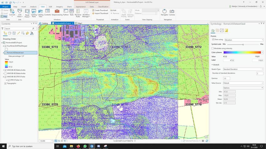
Abstract
Dutch
Het doel van dit onderzoek is het verder in kaart brengen van de geomorphologie van het
Baruth-oerstroomdal. Het onderzoek bouwt daarmee voort op het onderzoek dat vorig jaar is
uitgevoerd door bachelor studenten Geskus (2020), Nobel (2020), Luimes (2020), Romar
(2020), Schadee (2020) en Zuidervaart (2020). Het Baruth-oerstroomdal is gelegen in
Duitsland ten zuiden van Berlijn en gevormd in de laatste 2 ijstijden. De geomorphologische
kaart is gemaakt door middel van digitale bronnen zoals LiDAR data, luchtfoto’s en eerder
gemaakte kaarten. Verder is de geomorphologische kaart gemaakt in samenwerking met 3
onderzoekspartners, A. Melger (2021), H. van Gelderen (2021) en J. Wesselman (2021).
Hierbij zijn verschillende landvormen in kaart gebracht waaronder morenen, verschillende
oerstroomdalterassen, duinen, en een sander. Verder zijn er op basis van literatuur en de
geomorphologische kaart verschillende paleo-geografische kaarten gemaakt die laten zien
hoe het onderzoeksgebied er potentieel heeft uitgezien in 4 belangrijke fases van de
vorming van het landschap.

English
The aim of this research is to further map the geomorphology of the Central Baruther Ice-
Marginal valley. The research builds on research carried out last year by bachelor students
Geskus (2020), Nobel (2020), Luimes (2020), Romar (2020), Schadee (2020) and
Zuidervaart (2020). The Central Baruther Ice-Marginal valley is located in Germany south of
Berlin and formed during the last 2 ice ages. The geomorphological map was created using
digital sources such as LiDAR data, aerial photographs and previously created maps.
Furthermore, the geomorphological map was made in collaboration with 3 research partners,
A. Melger (2021), H. van Gelderen (2021) and J. Wesselman (2021). Various land forms
have been mapped, including moraines, various valley terraces, dunes, and a sander.
Furthermore, based on literature and the geomorphological map, several paleo-geographical
maps have been made that show what the research area may have looked like during 4
important phases of the landscape formation.

                                                                                         2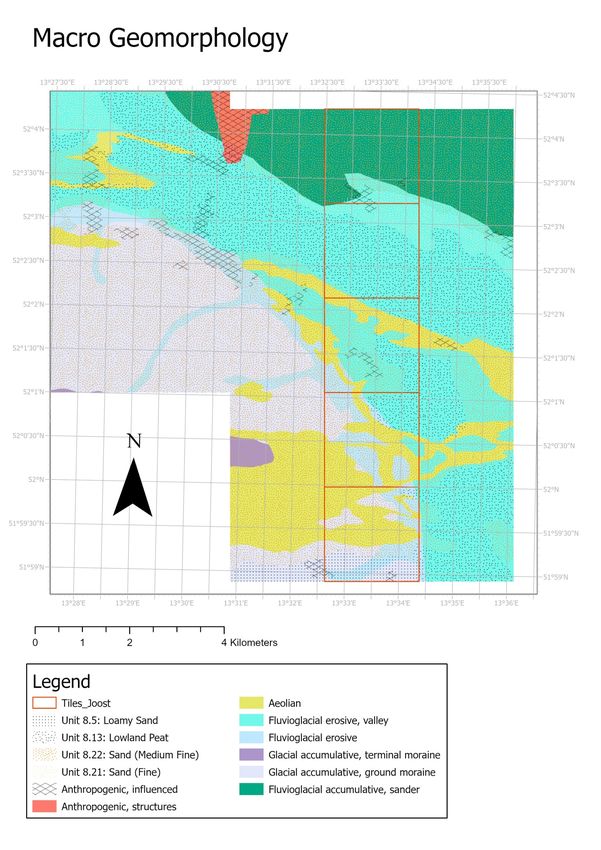
Contents

Inhoud
Abstract ...................................................................................................................................... 2
       Dutch................................................................................................................................... 2
       English ................................................................................................................................ 2
Contents ..................................................................................................................................... 3
Introduction ................................................................................................................................ 4
Methods and Data...................................................................................................................... 5
Results ..................................................................................................................................... 10
       1. Macro ............................................................................................................................ 11
       2. Meso ............................................................................................................................. 13
       3. Micro ............................................................................................................................. 15
       4. Other Results ................................................................................................................ 17
       5. Paleogeographic Maps................................................................................................. 21
Discussion ................................................................................................................................ 25
Conclusion ............................................................................................................................... 30
Literature .................................................................................................................................. 31
Acknowledgements .................................................................................................................. 32
Appendices .............................................................................................................................. 33
       Appendix A: Geomorphological map of the Central Baruth Ice-Marginal Valley. ........... 33
       Appendix B: Legend of the geomorphological map of the Central Baruth Ice-Marginal
       Valley. ............................................................................................................................... 34
       Appendix C: Overview of present features as created by research partner Melger
       (2021)................................................................................................................................ 35
       Appendix D: “Building an aprx project file for maps of the Baruth Ice-Marginal Valley in
       Brandenburg”. ................................................................................................................... 38

                                                                                                                                               3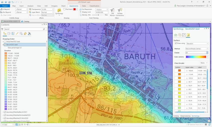
Introduction
Technological advancements that have taken place during the last few decades have led to
a massive increase in efficiency of many aspects of human life. The scientific community
and scientific research have greatly benefited from the abilities to share new information
worldwide with a few tabs of a button. Also technological advancements have made it
possible to measure and map the world around us in an incredibly efficient and precise way.
Traditionally geomorphological mapping was done through physical fieldwork which made
the mapping of larger areas labour intensive and therefore expensive (Jones, Brewer,
Johnstone, & Macklin, 2007). However, according to Geskus (2020) digitally mapping
geomorphological features based on LiDAR data can, despite having some limitations, to
some extent replace the traditional form of mapping through fieldwork.

Research Aims and Questions
In 2020 Geskus (2020), Nobel (2020), Luimes (2020), Romar (2020), Schadee (2020) and
Zuidervaart (2020) created a geomorphological map on macro, meso and micro level of the
Central Baruth Ice-Marginal Valley in Brandenburg Germany. The macro level contains
features that can be identified on a 1:100000 scale, the meso level contains features that
can be identified on a 1:10000 scale and the micro scale contains features that can be
identified on a 1:1000 scale.

Figure 1: Research area 2020, 2021 and research strip.

                                                                                             4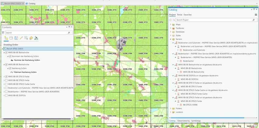
This map was based on the legends of the mappings of Pachur & Schulz (1983) and Frank
(1987). The main goal of this research is to expand that map eastwards using the same
legend and improving it where possible. This is done by relying on solely digital available
data like LiDAR data, existing maps and photos. Furthermore this research project is done in
collaboration with 3 research partners, Hein van Gelderen, Jaap Wesselman and Aletta
Melger. In order to reach the goal of this research geomorphological features must be
identified on macro, meso and micro level. The macro level contains features that can be
identified on a 1:100000 scale, the meso level contains features that can be identified on a
1:10000 scale and the micro scale contains features that can be identified on a 1:1000 scale.
Reaching the goal of this research will also require the following research questions to be
answered:

   - What geomorphological features, landforms and structures can be identified using
   LiDAR data, aerial photos and other digital sources?

   -   To what extent have people influenced the geological features in the research area?

Another goal of this research is the creation of several paleo-geographical maps of the
Baruth Ice-Marginal Valley on a macro scale. These maps will form a time line that shows
the four most important phases during the geomorphology of the research area, the Saalian
glaciation, the Eemian, the Weichselian glaciation and the current day situation. The goal
with these paleo-geographical maps is to help people who are not familiar with the research
area understand the geomorphology of the area. Furthermore it will form a basis for more
detailed paleo-geographical maps that could be made in the future.

Methods and Data
At the start of this project dr. W. M. de Boer, expert in the geomorphology of the study area,
discussed and explained the most important and prevalent landforms in the study area and
how they were formed. Afterwards more literature on the area has been studied, the most
important of which are de Boer (1995), Juschus (2001), de Boer (2015), Geskus (2020),
Nobel (2020), Luimes (2020), Romar (2020), Schadee (2020) and Zuidervaart (2020).
Thirdly, the e-learning courses from ESRI ‘Lidar in ArcGIS: an Introduction’, ‘Managing Lidar
Data Using LAS Datasets’, ‘Managing Lidar Data Using Terrain Datasets’ and ‘Managing
Lidar Data Using Mosaic Datasets’ have been completed to gain more knowledge about how
to use the LiDAR data and the software that was required for this research.

After this the “How to build an APRX” file that was provided by supervisor dr. W.M. de Boer
was used to create an ArcGIS Pro project file with the extension ‘.aprx’. The “How to build an
APRX” file describes which projections to use, how to add the most important existing maps
to the ‘.aprx’ file as well as how to turn the LiDAR data tiles into usable layers in the ‘.aprx’
file. The document also helped to create a similar basis for all of the previously mentioned
research partners. Which made transferring data between the research partners a lot more
efficient.

                                                                                               5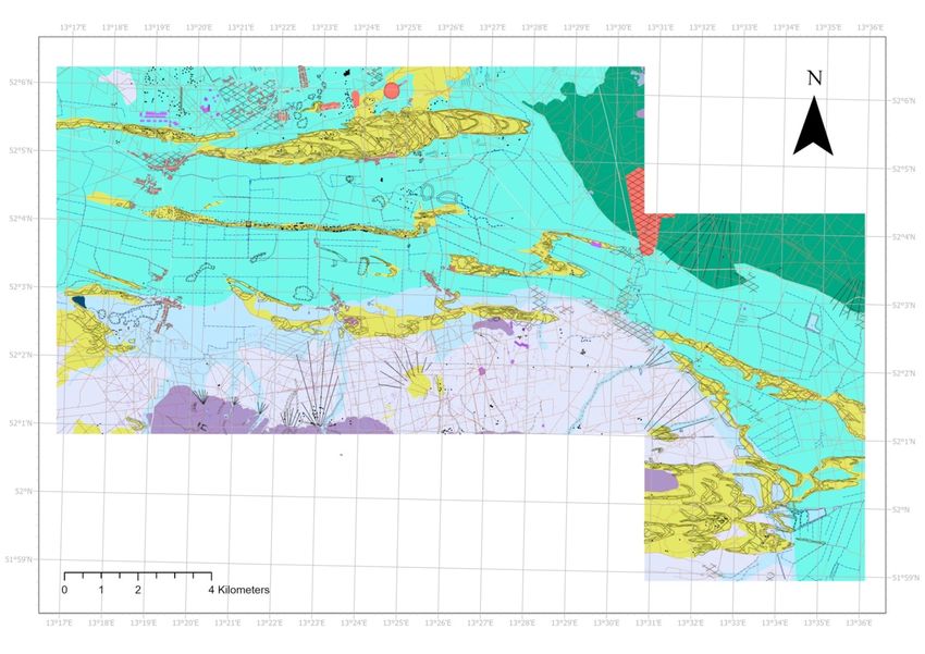
The most important data like the LiDAR tiles, previously made maps, photos and literature
was provided by dr. W.M. de Boer and was shared through surfdrive.nl. For the sharing of
data between the research partners Microsoft Teams was used. This was also used for
discussions through video calls which will be mentioned later.
The 30 LiDAR tiles that have been used for this research consist of xyz ascii files and
contain elevation data of millions of points forming a big point cloud of elevation data. These
files contain about 3 points per square meter and are transformed into ‘.LAS’ files from which
the digital elevation model (DEM) has been generated. This DEM file has a value for every
0.25 square meter and is therefore very accurate. This DEM file could then be used to create
different elevation derived maps such as a hillshade map, aspect map, contour map and
slope map. These were then used together with the DEM, literature, existing maps, photos
and satellite imagery to map the geomorphological features of the research area. Appendix
E contains a table that shows what sources and maps have been used to create certain
features.
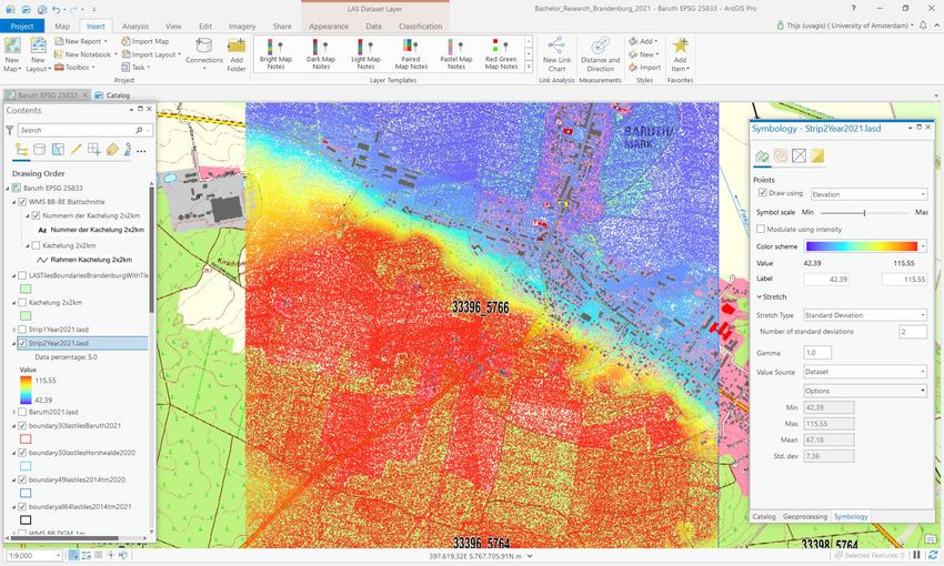
In order to locate and map important features of the area the dynamic range adjustment
(DRA) was used on the DEM. This adjusts the symbology of the DEM layer to the elevation
of the area within the screen window. This makes small, but sometimes important,
differences in the elevation visible. Figure 2 and Figure 3 both display the same part of the
research area, however in Figure 2 DRA is turned off whereas in Figure 3 DRA has been
turned on. Because of the DRA the dune formations are much better visible in Figure 3 than
in Figure 2. However both figures contain the same legend created by ArcGIS Pro which is
correct for Figure 2 but incorrect for Figure 3. This is because ArcGIS Pro uses the elevation
values of the entire DEM to create the legend instead of using the elevation values of the
displayed part of the DEM. Another tool to get a clearer image of features in the area is
convolution which research partner van Gelderen (2021) has described in more detail.
6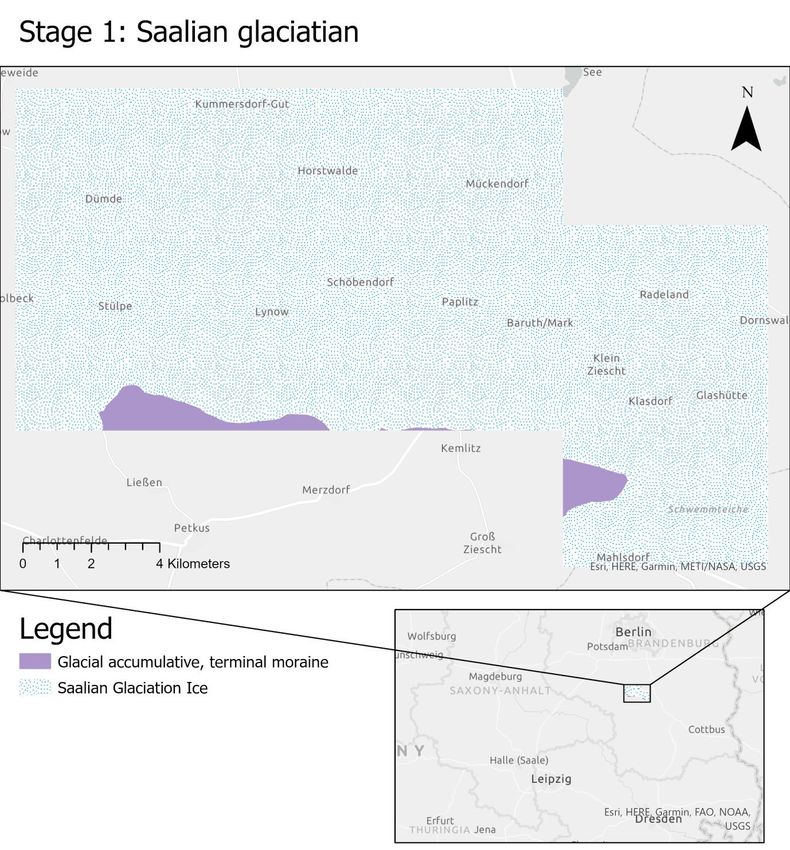
Figure 2: Dunes near Glashütte with DRA turned off.

                                                      7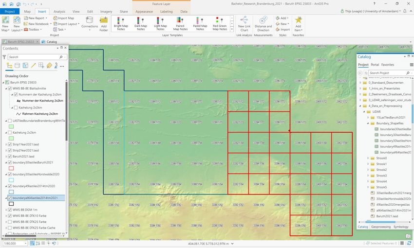
Figure 3: Dunes near Glashütte with DRA turned on. (Note that the legend is incorrect.)

The legend of the geomorphological map will, just like the legend made by Schadee (2020),
be based on the legend created by Frank (1987) and the legend created by Pachur &
Schultz (1983). According to Schadee (2020) the legend made by Frank (1987) is very
detailed and it contains classifications of most landforms that can be found in Germany.
Schadee (2020) also states that the legend created by Frank (1987) has been based on the
legend made by Pachur & Schultz (1983) which was made for a similar area as the Central
Baruther ice-marginal valley. However, according to Schadee (2020) the existing legends
needed some additions, like military point and line features, to better show the important
features of the research area. Therefore the legend created by Schadee (2020) will be used

                                                                                          8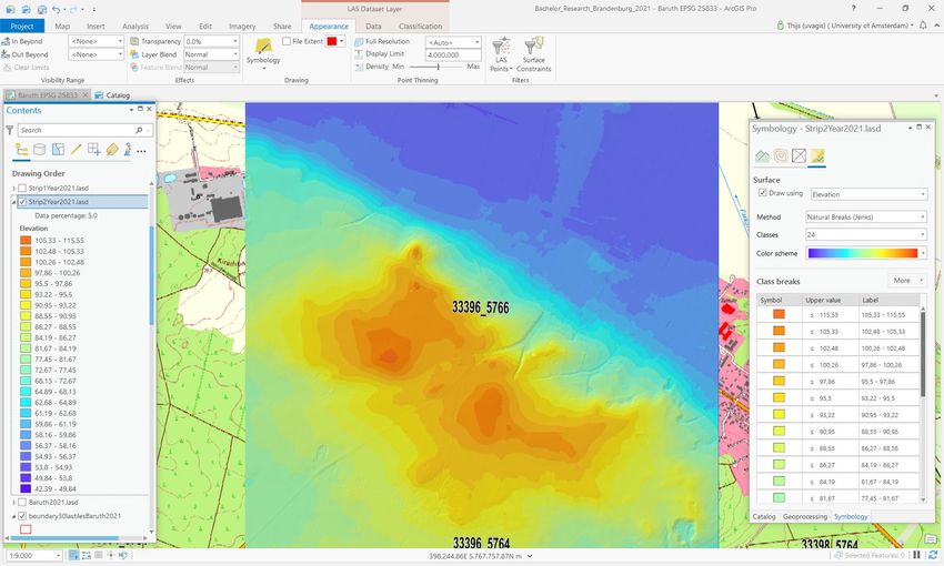
for the geomorphological map of this year and identified features that are not yet in that
legend will be added based on the legend created by Frank (1987).

In order to create the correct symbology to the geomorphological map Schadee (2020)
added codes to the features. These codes have been based on the classifications of the
legend. However the classifications in the legends use dots to differentiate between main
classifications, landforms and categories. The codes used for the symbology in ArcGIS Pro
cannot contain “.”. Therefore the “.” has been replaced by “0”. This means for example that
the legend unit 13.6 Fluvioglacial Accumulative will be marked with 1306 in the attribute
table on ArcGIS Pro as can be seen in figure 4.

Figure 4: Codes for Features in ArcGIS Pro.

To better utilize the possibilities of digital mapping the different features of last year's feature
class “Unit 13” of the macro geomorphology have been separated into different feature
classes. The goal of this adjustment was to be able to overlap some features creating a
more accurate representation of the geomorphology. Since the dunes and anthropogenic
structures lay on top of other geomorphological features such as ground moraines this was
the most accurate way to map these features. This also makes it possible to display only
certain features, for example showing just the ground moraines without the dunes on top.

According to Jones et al. (2007) the mapping of geomorphological features is often
subjected to interpretations and can be subjective. Therefore most of the mapped features
during this research have been discussed with multiple research partners.

The paleo-geological maps will be based on the macro geomorphological map and literature
research. And will therefore use the same legend as the geomorphological map.
Furthermore the different maps, each representing a different period, will be mapped as
feature groups so that they can be easily turned on and off separately.

After the research the results will be stored in the GIS studio of the University of Amsterdam
and published on Figshare.com. From there the data and results can be accessed by
potential beneficiaries. The maps created during this research have been collected in an
organized project file with all the important metadata. This will ensure that beneficiaries can
easily work with the created maps.

                                                                                                   9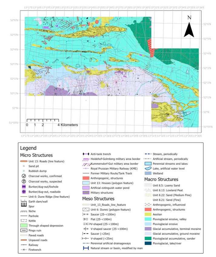
Results
This paragraph has been divided into 5 parts of which the first 3 will subsequently focus on
the macro, meso and micro structures that have been mapped in the fieldwork strip marked
as blue in figure 1. In these 3 parts all the mapped features will be focused on from north to
south. Other parts of the research area will be discussed by research partners van Gelderen
(2021), Melger (2021) and Wesselman (2021).The fourth part of this paragraph will focus on
some other results that do not directly fit within the other three parts and the fifth part will
focus on the paleo-geological maps.

Figure 5: Geomorphology map (Macro, Meso & Micro) of the research area in 2020 and
2021 of the Central Baruth Ice-Marginal Valley. For a higher resolution see Appendix A & B.

                                                                                              10
1. Macro
Figure 6: Overview of the Macro features of the research strip.
11As shown in figure 6 most of the northern part of the fieldwork area has been covered by the
Baruther Sander. The Baruther Sander mainly consists of medium fine sand which has been
deposited like a big alluvial fan by the melting ice masses in and shortly after the
Weichselian glaciation period and is therefore mapped as ‘Fluvioglacial accumulative’ (See
Appendix C for the corresponding units). On the edge of the sander the village Radeland can
be found which has been mapped as ‘Anthropogenic influenced’. When looking at the total
research area it becomes clear that humans have mostly built on the parts of the area that
contain a lot of sand. This land is less wet than the ice-marginal valley which has a lot of
lowland peat soils. The dryer sandy areas like the sander, dunes and moraines are also less
suitable for agricultural purposes because those areas are relatively dry and less fertile.
Later in time the Baruther Sander has been undercut by the ice-marginal valley (Juschus,
2001) creating a sharp threshold in the field and a sharp line on the map between the sander
and the ice-marginal valley marked with ‘B’ in figure 7.
Figure 7: A: The village of Radeland on top of an alluvial fan. B: Edge of the Baruther-
sander. (Notice that the elevation values shown in the legend do not represent meters.)
Moving south from the sander the ice-marginal valley can be found. This is the lowest and
wettest part of the research area and mainly consists of lowland peat soils. The ice-marginal
valley has mainly been formed by melting glacial water and is therefore mapped as
‘fluvioglacial erosive’ and ‘fluvioglacial erosive valley’ depending on the terrace level.
The south of the research area consists of ground moraines and terminal moraine which
have been formed by the ice masses during the saalian glaciation. The terminal moraines
12were formed right in front of the ice masses and therefore mark the furthest extension of the
ice masses during the formation of this area. The ground moraines were deposited from
underneath the ice mass and lay in between the ice-marginal valley and terminal moraines.
Since the ground and terminal moraines have been deposited by the ice masses they are
mapped as ‘glacial accumulative ground moraines’ and ‘glacial accumulative terminal
moraines’. Also the ground moraines have been undercut by the ice-marginal valley which
has caused sharp distinction between the elevation of both areas.
After the formation of the previously mentioned landforms aeolian processes have formed
dune formations on top of the ice-marginal valley, terminal moraines and ground moraines.
In the middle of the research strip on the ice-marginal valley there seems to be a longitudinal
dune formation. However when looking on a smaller scale some parabolic dunes can be
distinguished which have been heavily affected by anthropogenic processes. Further south
parallel to the ground moraines a remarkable dune formation can be seen which will be
discussed in the fourth part of this paragraph and in the discussion. Even further down a big
dune formation, consisting of several large and small parabolic dunes, covers the terminal
moraines, ground moraines and ice-marginal valley.
2. Meso
On a meso level the first thing to be seen in the north of the research area are the small v
shaped valleys leading from the sander to the lower ice-marginal valley. These v-shaped
valleys have been formed by melting water from the glacier during the Weichselian
Glaciation. A little bit further south on the border between the sander and the ice-marginal
valley a main road can be found which has likely been built there for the same reason most
buildings are built near dunes, the sander or the moraines. The dry sands are more suited to
build on than the wet ice-marginal valley. In the ice-marginal valley a lot of perennial artificial
drainage ways can be found which are used for the agricultural activities in the ice-marginal
valley. Just like on the macro scale dunes have been mapped on a meso scale. However the
meso scale has been focused on individual dunes instead of aeolian affected areas. Also in
the south of the research area strip dunes have been identified, however these show much
more clearly the parabolic shapes than the dunes found in the middle of the ice-marginal
valley. Furthermore the south contains a wide v-shaped valley leading from the ground
moraines to the ice-marginal valley. Also another main road can be found running parallel to
the ground moraines for the same reason as previously mentioned. Just east of the most
southern tile of the research strip lay several ponds that are being used for the breeding of
several fish species like carp and pike. These ponds can also clearly be seen on the
hillshade map and DEM because of the dikes that surround them.
13Figure 8: Overview of the Meso features of the research strip.
143. Micro
Figure 9: Overview of the Micro features of the research strip.
15The most prevalent features on a micro scale in the north of the research area strip are the
roads. Most roads are located on the sander to provide access to some tiny houses on the
sander or to accommodate forestry. Another prevalent feature in the north of the research
area is the big alluvial fan that runs from the sander onto the ice-marginal valley. The village
Radeland is also built on top of this alluvial fan. Within a small valley in the alluvial fan a
suspected Relict Charcoal Work (RCH) has been mapped. And a kettle, a depression in the
landscape caused by the melting of a detached piece of glacial ice, can be found somewhat
east of the alluvial fan still on the Baruther Sander. Further south onto the ice-marginal valley
a military structure has been mapped which, based on the shape and size, may have been
used as an artillery station during the second world war. Straight south from this military
structure some earth dams/walls have been mapped. Since the earth dams are located in a
forest area the purpose is somewhat unclear and requires more research. On micro scale
the ridges of the dunes have been mapped which clearly show the different dune types in
the research area. Starting with a combination of longitudinal and small parabolic dunes on
the ice marginal valley that have been excavated to make way for roads and for the glass
production in the village Glashütte which is located just east of the research strip. Further
south parallel to the ground moraines are the somewhat pointy shaped dune formations that
will be mentioned later. All the way in the south of the area the parabolic dunes are clearly
visible by the ridges of the dunes. In the south of the research strip also more suspected
charcoal hearts are mapped.
164. Other Results
Paleo rivers
In the south of the research strip something that looks like two very small paleo rivers have
been found which can be seen in figure 10. However due to the small size they could also be
drainage ways for rainwater that runs from the terminal and ground moraines to the valley.
Due to the inaccuracy of the profile function in ArcGIS Pro a no profile could be made of this
potential paleo river. This will be further explained in the discussion.
Figure 10: Small potential paleo river visible on DEM.
However further to the east in the research area a much bigger paleo river has been
identified (figure 11). According to de Boer (personal communication, 7-4-2021) this must be
the old Dahme river. It can also clearly be seen how originally the river ran north but it has
been cut off by the dunes that formed later. In this way the old Dahme river was forced to
bend to the east in a sharp curve. This is the case just north of the area depicted in figure
11. The profile graph that can be seen in figure 12 shows that the paleo river Dahme is
about 30 centimeters lower than the surrounding area. However, as will be explained in the
discussion, these profile graphs are not very accurate.
17Figure 11: Paleo river Dahme as seen on the DEM.
Figure 12: Profile graph of the paleo river Dahme.
18Spit-like dunes
Parallel to the ground moraines in the south of the ice-marginal valley, dunes can be found
which do not match the description of the parabolic or longitudinal dunes like the other dunes
in the research area. The crest of the dunes seems to run parallel to the ground moraines
and the dunes seem to have some northeast facing teeth like shapes. The appearance of
these dunes seems to be somewhat similar to that of spit dunes which are found in coastal
delta regions. However these can’t be identified as spit dunes because the ice-marginal
valley has never been a coastal region. Possible explanations for the formation of these
remarkable dunes can be found in the discussion.
Figure 13: Spit dunes in a deltaic coast. (Ranwell, 1977)
19Figure 14: Unidentified dunes in the research area.
Mistake in legend 2020
One of the goals of this research was to improve the legend for the geomorphological map
that had been created by Schadee (2020). One of the required improvements was the
addition of the legend unit ‘fluvioglacial accumulative’ to correctly map the sander in the
north east of the research area. Like described in the methods, additional legend items
would be based on the legend created by Frank (1987). However, the code for ‘fluvioglacial
accumulative’ was ‘13.6’ in the legend of Frank (1987), which had been used by Schadee
(2020) for ‘fluvioglacial erosive’. This was most likely done to differentiate between different
terrace levels of the ice-marginal valley and didn’t form an issue since no fluvioglacial
accumulative landforms were present in the research area of 2020. In order to solve this
issue the two terrace levels have been split up into ‘13.7.1’ and ‘13.7.2’ leaving ‘13.6’
available for ‘fluvioglacial accumulative’.
205. Paleogeographic Maps
The first paleo-geographic map named “stage 1” represents the research area during the
Saalian glaciation, see figure 15. During this period ice sheaths covered almost the entire
research area creating the terminal moraines at the front of the ice sheaths and the ground
moraines underneath the ice sheaths.
Figure 15: Paleogeographic map stage 1 representing the research area during the Saalian
Glaciation.
21The second paleogeographic map named “stage 2” represents the Eemian period during
which the ice sheaths covering the research area had melted away and left behind the
terminal and ground moraines, see figure 16.
Figure 16: Paleogeographic map stage 2 representing the research area during the Eemian
Period.
22Figure 17 named “stage 3” represents the research area during the Weichselian glaciation
during which ice covered the area just north of the research area. Melting water from these
ice sheaths created the Baruther Ice-Marginal valley as well as the Sander in the north east
of the research area. Furthermore erosive processes have been going on for longer which
can be seen in the ground and terminal moraines.
Figure 17: Paleogeographic map stage 3 representing the research area during the
Weichselian Glaciation.
23Figure 18 shows the last paleo-geographical map which represents the current situation of
the research area. At this time several dune formations have formed in the research area.
Also humans have greatly influenced the area by building towns and other structures.
Figure 18: Paleo-geographical map stage 4 representing the research area as it is today.
24Discussion
No fieldwork possible
Due to Covid-19 related travel restrictions during this research it has not been possible to do
fieldwork in the research area. According to Geskus (2020) it is important to check digitally
mapped features in the field to increase the reliability of the geomorphological map.
Especially smaller landforms like military structures and relic charcoal works are difficult to
identify with a high certainty using sole digital sources. However also the marco features
could be mapped more accurately if fieldwork would have been possible since most of the
digital data only provides information on the top layer of the surface while a more accurate
map would require some knowledge of underlying layers in the soil. Checking this years'
mapped geomorphological features in the field is something that could be done in future
research.
Mapping Dunes
According to Hugenholtz et al (2012) the mapping of dunes using remote sensing data like
LiDAR can be very subjective and offers room for interpretations. To adjust for this the dunes
in the research area have been mapped in three different ways on macro, meso and micro
level, showing the total aeolian influenced area’s on macro level, the dune shapes on meso
level and the ridges of the dunes on micro level. However, like figure 19 shows within these
levels there is still room for different results.
Figure
19: “Defining the boundaries of sand dunes for the purpose of spatial analysis can add a
high degree of subjectivity to the outcome. Here we show two contrasting interpretations of
the boundaries of dunes at White Sands, New Mexico, USA.” (Hugenholtz et al. 2012. page
329)
25Spit-like Dunes
The oddly shaped dunes running parallel to the ground moraines which have previously
been mentioned could potentially be explained by a few processes which have taken or are
still taking place in the research area. As previously mentioned the shape of the dunes
shows similarities with that of spit dunes formed in a deltaic coast. Despite this not being a
coastal region it might have been a delta which formed from the erosive valleys in the
Saalian ground moraines in the south west. This argument might be substantiated by the
fact that these dunes are found directly in line with two very big erosive valleys in the
moraines. However they do not seem to be present near other valleys in the ground
moraines. Something else that might have played a role in the formation of these dunes are
bidirectional winds. The North-South and East-West directions of the arms of the dunes
suggest winds from the north and east which could have been possible. During the glacial
and early periglacial periods which have shaped most of the landforms in the research area
the wind was most likely predominantly coming from the east. According to de Boer
(personal communication, 28-5-2021) this was the case because of the ice masses in the
north east causing a high pressure zone in comparison to the warmer south west. When the
ice masses were close to the research area the wind direction was most likely predominantly
north. But when the ice masses retracted further north the wind direction got predominantly
east because of the Coriolis effect. After the glacial periods this wind direction has changed
to being predominantly west. Another remarkable feature of these dunes are the steep
slopes on the north and east side and the relatively shallow slope on the south and west
side. Some dune types like barchan dunes naturally have a steeper side facing the same
direction as the wind is blowing. In this case that would suggest winds from the south-west.
However there could also be several other reasons for the steeper north and east sides. Just
like fluvio-glacial erosion from water in the ice-marginal valley undercut the moraines and
sander it could, in a later stadium, also have undercut the dunes on the sides facing the ice-
marginal valley. Another explanation would be excavation by humans. According to de Boer
(personal communication, 28-5-2021) sand was a useful material to stabilize the wet peat
soils or make peat soils more fertile in the ice-marginal valley. For this reason most of the
anthropogenic structures like villages and cities in the research area are found on or near
Aeolian influenced locations.
26Valley Terraces
According to Juschus (2001) the ice-marginal valley has 4 different terraces of which the
highest and oldest are in the south, and the lower and younger terrasses are in the north.
Figure 20: 4 different terraces in the Central Baruther Ice-Marginal valley. (Juschus, 2001)
Two of these terraces could easily be identified and have been mapped on the
geomorphological map. In order to map the 4 river terraces that Juschus (2001) mentions,
multiple cross sections of the ice-marginal valley have been made. However despite the
accuracy of the DEM ArcGIS Pro didn’t give an accurate result making it hard to distinguish
different terraces. This issue can also be seen in figure 21 where a profile has been created
of a part of the paleo river Dahme. The profile has been created based on the DEM that
contains elevation data for every 0.5 meters. The profile covers a length of about 50 meters
and should therefore contain about 100 elevation values. Instead the profile only seems to
displays 4 values creating a super inaccurate profile. In this case it even results in a profile
graph that seems to display a small increase in height where the paleo river is located while
the DEM clearly shows the middle of the profile should be lower than the ends of the profile.
27Figure 21: Screenshot taken on 09-8-2021 of a very inaccurate profile within ArcGIS Pro.
Furthermore ArcGIS Pro lacks a function that shows the corresponding location in the cross
section to the location on the map. Google Earth Pro does include a function that shows a
corresponding location on the cross section and the map which can be seen as the arrow in
in the top window and the bold vertical line in the lower window of figure 22. Unfortunately
using Google Earth pro didn’t give an accurate result either because the elevation data didn’t
seem accurate and seemed to be heavily affected by trees and houses. As can be seen in
figure 22 Google earth only displays the elevation in meters and is therefore not accurate
enough to clearly distinguish the 4 different terraces. Meaning that the 4 different terraces
as described by Juschus (2001) could not easily be distinguished with the methods
described in this research. The methodology described by research partner van Gelderen
(2021), which uses the convolution tool and dynamic range adjustment (DRA), might be
more effective to make a distinction between the different terraces.
28Figure 22: Screenshot taken on 09-08-2021 from Google Earth Pro. The top window is
displaying several lines from which a profile had been created. The lower window is
displaying the profile from line 6.
Separating Feature Class
As mentioned in ‘methods and data’ last year's feature class “Unit 13” containing macro
geomorphological features has been separated into different feature classes to improve the
accuracy by accommodating overlapping features. However this adjustment also came with
some challenges. The first of which is accurately mapping geomorphological features that
are covered by another feature. For example a dune can lay on top of terminal moraines and
ground moraines which makes it hard to map the exact border between the moraine types.
This is especially difficult when using digital sources only. This means that this adjustment
has made the map better at representing the situation but that it also has created some less
accurate spots in the map where multiple features overlap each other. A second challenge
that has been caused by this adjustment is that features can no longer be mapped by
splitting them from one big polygon. This means that features have to be created from their
own separate feature class and snapped to other features to create a fully covered map.
This makes the workflow more time consuming and more sensitive to drawing errors.
29DRA
As mentioned previously Dynamic Range Adjustment (DRA) is a tool in ArcGIS Pro that
adjusts the symbology to the values of the present features in the screen window. DRA has
been used intensively during this research because it helped to identify small but important
differences in the elevation of the area, like for example the paleo river Dahme. However
DRA comes with some disadvantages regarding the visualization of values. When a map
layout is being created of a part of a Digital Elevation Model (DEM) the DRA will adjust the
symbology making elevation differences more visible. However when a legend is added to
the layout it will contain values for the entire DEM instead of the values present in the
selected window. Therefore colors show in certain maps would not correspond to the legend
generated by ArcGIS Pro. The result is that layouts that contain a DEM with DRA only show
the relative elevation of the displayed area instead of absolute elevation values. This issue
could potentially be solved with an option to adjust the legend to the values of features
present in the layout window. However that option could not be found in ArcGIS Pro during
the extent of this research.
Paleo-Geographic maps
The paleo-geographic maps that have been created during this research show what the
research area might have been like during the mentioned periods. However, it is not possible
to create a map that shows the exact situation at a certain point in history. The first reason
for this is that the geologic situation was not constantly the same during one of the
mentioned periods. For example, ice sheaths during the glaciations grew and shrunk
depending on the years and seasons. Furthermore the paleo-geographic maps have only
been based on literature research and the geomorphological map made during this
research. These two sources seem to provide a decent view on what the research area
might have looked like during the mentioned periods, however they do not provide enough
detailed information to create an accurate map of a certain point in time.
Conclusion
To conclude a geomorphological map has successfully been created showing the
geomorphology of the research area on a macro, meso and micro scale. Some dune
formations could not be identified as a certain dune type but show resemblance with spit
dunes found in coastal regions. There are also multiple potential explanations for the
formations of these dunes. Because traveling to the research area during this research was
not possible, not all identified features can be confirmed. This should be done in future
research to make the created map more reliable. Furthermore 4 paleo-geographical maps
have been created. These maps show what the research area might have looked like during
4 important stages of the formation of the landscape of the area.
30Literature
Boer, W.M. de (1992a). Äolische Prozesse und Landschaftsformen im mittleren Baruther
Urstromtal seit dem Hochglazial der Weichselkaltzeit. Berlin, Humboldt-Universität,
Dissertation, 144 p. & Anhang 75 p. DOI: http://dx.doi.org/10.18452/13573
Boer, W. M. de (1992b). Form und Verbreitung der Dünen im Gebiet zwischen Luckenwalde
und Golssen (Niederlausitz). Berlin, Humboldt-Universität. DOI:
http://dx.doi.org/10.18452/13452
Boer, W.M. de (1995): Äolische Prozesse und Landschaftsformen im mittleren Baruther
Urstromtal seit dem Hochglazial der Weichselkaltzeit. Berliner Geographische Arbeiten, 84:
S. 1 - 215, Based on Dissertation from 1992, Humboldt Universität zu Berlin. DOI:
https://doi.org/10.18452/13573
Boer, W.M. de (1999): Dünen um Glashütte bei Baruth. Gutachten für Natur und Text in
Brandenburg, Rangsdorf, 16 Seiten Text, 21 Seiten im Anhang.
http://www.kaartopmaat.eu/D/Publikationen/1999/Gutachten_zu_den_Duenen_um_Glashuet
te_bei_Baruth-WMdeBoer1999.pdf
Boer, W.M. de (2015). W.M. de Boer: Eine reliktische Parabeldüne und Wölbäcker im
Baruther Urstromtal westlich von Schöbendorf entdeckt durch Laserscandatenauswertung. -
In: Biologische Studien. - Luckau 44, blz. 4 - 12. ISSN: 1432-4199. DOI:
https://doi.org/10.18452/13669
Boer, W. M. D. (2016). Eine reliktische Parabeldüne und Wölbäcker im Baruther Urstromtal
westlich von Schöbendorf entdeckt durch Laserscandatenauswertung. DOI:
http://dx.doi.org/10.18452/13669
Frank, F. (1987). Die Auswertung grossmassstabiger Geomorphologischer Karten (GMK 25)
fur den Schulunterricht. Berliner Geographische Abhandlungen, 46(Gmk 25).
https://doi.org/10.23689/fidgeo-3192
Van Gelderen, H. (2021) The reliability of digital classification and mapping of the Baruth Ice-
marginal valley. (unpublished bachelor thesis). University of Amsterdam, Amsterdam,
Netherlands.
Geskus, S. (2020) The reliability of geomorphological mapping using LiDAR data: the
Central Baruth Ice-Marginal Valley (unpublished
bachelor thesis). University of Amsterdam, Amsterdam, Netherlands. Retrieved from
http://www.gisstudio.nl/index.php?page=bsc#geskus
Hugenholtz, C. H., Levin, N., Barchyn, T. E., & Baddock, M. C. (2012). Remote sensing and
spatial analysis of aeolian sand dunes: A review and outlook. Earth-Science Reviews,
111(3–4), 319–334. https://doi.org/10.1016/j.earscirev.2011.11.006
Juschus, O. (2001). Das Jungmoränenland südlich von Berlin - Untersuchungen zur
jungquartären Landschaftsentwicklung zwischen Unterspreewald und Nuthe. Dissertation.
Humboldt-Universität zu Berlin. https://doi.org/10.18452/14585
31Jones, A. F., Brewer, P. A., Johnstone, E., & Macklin, M. G. (2007). High-resolution
interpretative geomorphological mapping of river valley environments using airborne
LiDAR data. Earth Surface Processes and Landforms, 32(10), 1574–1592.
https://doi.org/10.1002/esp.1505
Luimes, B.J. (2020) The adequacy of digital geomorphological research - Research into the
adequacy of digital geomorphological conducted research by creation of a
geomorphological map and identification of ridge and furrow-systems, for Horstwalde,
Germany. University of Amsterdam, Amsterdam, Netherlands. Retrieved from
http://www.gis-studio.nl/index.php?page=bsc#Luimes
Melger, A. (2021) The creation of a geomorphology map and the identification of the paleo
drainage system of the Hammerfließ stream in the Central Baruth Ice-Marginal Valley with
the use of LiDAR Data. (unpublished bachelor thesis). University of Amsterdam, Amsterdam,
Netherlands.
Pachur, H. & Schulz, G. (1983). Erläuterungen zur Geomorphologischen Karte 1:25 000 der
Bundesrepublik Deutschland GMK 25 Blatt 13, 3545 Berlin-Zehlendorf, P. 1-88.
Romar, M. (2020) Digitally mapping the geomorphology of the Baruth Ice-Marginal Valley,
Germany (unpublished bachelor thesis). University of Amsterdam, Amsterdam,
Netherlands. Retrieved from http://www.gis-studio.nl/index.php?page=bsc#romar
Ranwell, D.S. & Boar, R., (1977). Coast dune management guide. Institute of Terrestrial
Ecology, HMSO, London.
Schadee, M. (2020). Creating a geomorphological map of a formerly glaciated area in
Brandenburg, Germany (unpublished bachelor thesis). University of Amsterdam,
Amsterdam, Netherlands. Retrieved from
http://www.gisstudio.nl/index.php?page=bsc#Schadee
Wesselman, J. (2021) Geomorphological mapping and tracing of paleo-river systems in
Baruth Ice Marginal Valley, Brandenburg, Germany – By use of LiDAR data, satellite images
in ArcGIS Pro and conventional geological data. (unpublished bachelor thesis). University of
Amsterdam, Amsterdam, Netherlands.
Zuidervaart, S.J.C (2020) The creation of a large scale Geomorphological map of the Central
Baruth Ice-Marginal Valley, Germany (unpublished bachelor thesis). University of
Amsterdam, Amsterdam, Netherlands. Retrieved from
http://www.gisstudio.nl/index.php?page=bsc#zuidervaart
Acknowledgements
First I would like to thank dr. W.M. de Boer for providing an incredible amount of data and
information about the area, providing feedback, meeting and discussing multiple times
during the research and helping to move the research in the right direction. Secondly I would
like to thank research partners Jaap Wesselman, Aletta Melger and Hein van Gelderen for
the pleasant teamwork during this research. Furthermore I would like to thank the University
of Amsterdam for providing the ArcGIS Pro License and elevation data required for the
research.
32Appendices
Appendix A: Geomorphological map of the Central Baruth Ice-Marginal
Valley.
33Appendix B: Legend of the geomorphological map of the Central Baruth
Ice-Marginal Valley.
34Appendix C: Overview of present features as created by research
partner Melger (2021).
3536
37
Appendix D: “Building an aprx project file for maps of the Baruth Ice-
Marginal Valley in Brandenburg”.

      Building an aprx project file for maps of the
      Baruth Ice-Marginal Valley in Brandenburg
This workflow will go through the steps to generate an .aprx file for use in ArcGIS Pro with web
services and local geodata, partly downloaded from the UvA Geoportal or from the Surfdrive for the
Bachelor Project under supervision of Thijs de Boer. Part of the maps that we will insert/use are also
to be found at: https://bb-viewer.geobasis-bb.de/ (=Brandenburgviewer) and at

http://www.geo.brandenburg.de/lbgr/bergbau (= Bergbauviewer) and

https://geobroker.geobasis-bb.de/ (general Site of Geobroker, the Internetshop of the LGB
(Landesvermessung und Geobasisinformation Brandenburg), for Topographical Maps:
https://geobroker.geobasis-bb.de/

WORKFLOW

    1. Start ArcGIS Pro. Check if you have the licenses for the extensions. You can do this by clicking
       project and checking under licensing. Check if you have the Spatial analyst, 3D analyst and
       Data Interoperability licensed. If not contact your ArcGIS manager = Thijs de Boer.

    2. Go back to the start screen > New > Blank Templates > Map.
    3. Create a New Project and call it ‘Bachelor_Research_Brandenburg_year_name’ (and check
       ‘Create a new folder for this project’).

                                                                                                    38
4. In the Contents Pane, Right click ‘Map’ > Properties > in Tab General change the name of the
Map to ‘Baruth EPSG 25833’.
5. In the same dialog box, head to > Coordinate Systems. Click (activate) – if necessary - the
rectangle beneath ‘Current XY’. In the Search box behind XY Coordinate Systems Available,
type in 25833 and click . The coordinate system ETRS 1989 UTM Zone 33N for XY will
appear blue in the search results (the number 25833 is an international EPSG number for
easy search of coordinate systems, like you used 25830 for Murcia in Spain). For more
information on this coordinate system: ETRS89 / UTM zone 33N - EPSG:25833. Do not close
the dialog box.
6. In the same dialog box, click ‘Current Z’. Type in the search box 5783 and click . This
will show you the DHHN92 vertical coordinate system (these refer to the height or Z-values
in your .las-datasets). For more information on this coordinate system: DHHN92 height -
EPSG:5783. Click OK.
397. Click on the Insert window > Connections > New WMS Server.
8. Add WMS Server (make sure to also copy the question mark ‘?’):
https://isk.geobasis-bb.de/ows/dtk25farbe_wms?
(This is a very actual kept topographical web map WMS, German scale 1:25.000).
9. In the Main Ribbon (top most ribbon), click View. Open a Catalog Pane.
10. In the list, Click Servers, so the new WMS connection shows up.
11. Expand the WMS connection (click the small triangle sign in front of the service name)
12. Drag and drop the WMS-DNM link WMS BB-BE DTK25 Farbe to your map.
13. Zoom to Baruth/Mark, set your Map scale at 1:100.000 and keep Baruth in the middle of
your map (the northern part of Golssen in the south should still be visible on your map). This
bookmark makes it easier for you to go back to this overview later if wanted.
14. Choose Map > Bookmarks > New Bookmark > Name: Baruth 1:100.000.
15. Now you can remove the ‘World Topographic Map’ and the ‘World Hillshade’ from your
TOC.
16. In the same manner, add these WMS from https://geobroker.geobasis-bb.de/ (there are also
WFS services for these maps, of which we will use some of them later) to your WMS Server
connections and to your map:
https://isk.geobasis-bb.de/ows/dtk10farbe_wms? (This is a topographical web map
1:10.000).
https://isk.geobasis-bb.de/mapproxy/dtk25farbe/service/wms? (This is a topographical web
map WMS, very quick, because it is cached, German scale 1:25.000).
17. Add also the WMS
https://inspire.brandenburg.de/services/bokarten_wms? (this is a soil map)
https://inspire.brandenburg.de/services/boartsubstr_wms? (a substrate map)
https://isk.geobasis-bb.de/ows/dop20c_wms? (these are aerial images in 20 cm resolution)
18. Add also the WMS https://isk.geobasis-bb.de/ows/dgm_wms? from the website DGM -
Produktmetadaten | Geobroker - Der Internetshop der LGB (geobasis-bb.de) to your Catalog
Pane and your map. This is a Digital Elevation Model (DEM) or in German: Digitales
Geländemodell (DGM).
40DSM = Digital Surface Model = would follow the highest points of the DEM.
19. Save your project. Do this regularly, in case the program crashes you have a recent copy at
least. Even better is to give your .aprx a new version name, e.g. the date of the day of last
edits.
20. It can come in handy that you have the tile numbers and tile borders at hand. We will add a
WMS and a WFS for this purpose. Each with advantages and disadvantages.
21. Add the following WMS to you map: https://isk.geobasis-bb.de/ows/blattschnitte_wms?
This WMS contains the tiles of maps and LiDAR data and according numbers (‘Blattschnitte &
Kachelung’). Add the layers ‘Kachelung 2x2 km’ and ‘Nummern der Kachelung’to your TOC as
top layer. Hint: tile numbers will not be shown when zoomed out beyond about 1:75.000.
4122. Your TOC, Catalog and map will now / should now look like (Baruth in the middle of your
map):
23. The WMS of the Tile numbers and tile boundaries is not very clear (a bit blurry). Add the
alternative Webservice, as a WFS to your Catalog Pane: Insert > Connections New WFS
Server. https://isk.geobasis-bb.de/ows/blattschnitte_wfs? Drag and drop the layer
‘Kachelung 2x2km’ to your map.
24. It is possible export the features of this WFS from the server in Brandeburg to your
geodatabase, because a WFS streams all the points, lines and polygons it contains.
Right-click on Kachelung 2x2 km in your TOC > Data > Export Features. Call the new feature
class ‘LASTilesBoundariesBrandenburgWithTileNumbers’. Check under ‘Environments’ that
you use the right projection (do this always in these kinds of dialog boxes in ArcGIS Pro).
42Zoom to layer. You will see that only in the western part of Brandenburg the webservice is
shown. Let’s hope, this is only a temporary problem!
25. The las files that you will use in this Bachelor Research were generated from the original xyz-
files that were bought by the UvA from the LGB = ‘Landesvermessung und
Geobasisinformation Brandenburg’ (https://geobasis-bb.de/lgb/de/) with the program
LAStools, with the command (sub program) txt2las (C:\LAStools\bin\txt2las.exe). In this
conversion, the coordinate systems EPSG 25833 (ETRS 1989 UTM Zone 33 North =
horizontal) and EPSG 5783 (DHHN92 = vertical) were implemented already, so you don’t
have to do that yourself. But the LAStools can also come in handy for other conversions and
creation of Land Surface Parameter products (e.g. hillshade, aspect, etc.), so please copy the
folder LAStools as a whole from the Surfdrive under the folder Software to the C-drive of
your laptop or home computer. The tools under the bin directory should work immediately,
without additional installing. Some tools have a windows interface, some others have a
command line interface and some tools have both.
4344
26. You should have received access to files and folders on the Surfdrive of Thijs de Boer:
    BSc Research Horstwalde 2020 en 2021 - Bestanden - SURFdrive
    One of those folders, beneath ‘Data’ is: ‘LiDAR Tiles 2021’ and it contains 6 strips (‘stroken’)
    with each 5 las files, covering each 2x2 km. So each strip is 10 km N-S and 2 km E-W.
    Strips 1 – 4 are assigned to you personally. N.B.: Strip 0: has been worked on in 2020 by Stef
    Zuidervaart and will be used for alignment purposes. Strip 5: has not been worked on in
    2020 and will be used for alignment purposes in 2021.

    Strip      Name Strip      Name student
    0          Schöbendorf     Stef Zuidervaart (2020)
    1          Paplitz         Jaap Wesselman
    2          Baruth          Aletta Melger
    3          Klein-Ziescht   Hein van Gelderen
    4          Klasdorf        Joost Bakker
    5          Glashütte       Extra (for alignment)

27. The folder ‘LiDAR Tiles 2020’ contains the 49 that were bought by the UvA before 2020,
    with a shapefile of the bounding box around those 49 tiles and another shapefile with the
    bounding box of the 30 tiles that were used by the students in 2020. And it contains sub-
    folders with a DEM per tile. The folder ‘LiDAR Tiles 2021’ also contains an overview shapefile
    of the 6 strips that will be used in 2021. Add all of the overview shapefiles to your GDB.
    Right click your GDB select import feature class. Don’t forget to name your output feature
    class.
        a. Beware: a shapefile consists of several files (not only .shp but also .dbf, .sbn, and so
             on)

                                                                                                 45
b. If you’re getting an error message you have to define a projection:
ETRS_1989_UTM_Zone_33N (=EPSG 25833).
Change the symbology to a 100% transparancy/change the color type to black or blue or
red outline (border).
N.B. the overview shapefile was made by using the tool ‘lasboundary.exe’ to extract the
outer boundary as a shapefile, with the command (see to it that you also fill in the projection
tab):
4628.
Make the shapefiles transparent (hollow) and use blue or black (tiles 2020) or red (tiles
2021) outline. See screen shot of map above. Now right-click on
‘boundaryall64lastiles2014tm2021 and ‘ zoom to layer’. Add an extra zoom layer of 1:90.000
in the box in the lower left corner:
29. Make a bookmark for this layer and another one for the ‘boundary30lastilesBaruth2021’
layer.
30. From the Surfdrive, download your assigned 5 LiDAR tiles. Field strips are assigned, see the
map of the field strips on page 5 of this document.
31. Create a new las dataset in the Catalog Pane or use the tool Create a Las Dataset and give it
the name StripNumberYear2021.lasd
a. Add your personal LAS files to the dataset.
b. Make sure to calculate statistics.
32. Assign a horizontal coordinate system to your personal las dataset: ETRS 1989 UTM Zone
33N = EPSG 25833.
4733. Assign a vertical coordinate system to your personal las dataset: DHHN92 = EPSG 5783.
34. Use the tool ‘Build LAS Dataset Pyramid’ for your personal las dataset.
35. Add your las dataset to the TOC.
36. Add an extra zoom layer of 1:9.000 in the box in the lower left corner.
37. Zoom in on one of your las tiles at a scale of 9,000. You should get a similar map view as the
images below:
4838. Make a visualization of the las dataset on the base of the elevation. In order to do this you
need to click one of the Lasd datasets in your TOC. Next click the appearance header (on the
top, in the main ribbon) and click on Symbology > Symbolize your layer using a surface >
Elevation. By doing this your dataset will create intervals. It should look similar to the image
below.
4939. Instead of the 9 default classes we would like to have 24. Head over to symbology by right
clicking the PersonalLasDataset in TOC. From the symbology screen change the amount of
classes to 24. ArcGIS Pro should assign proper spacing by itself. Choose a proper color
scheme.
40. Add the following (scanned, already georeferenced and very detailed) Military Topographical
Maps 1:25,000 from the 1980’s: Surfdrive > Data > Brandenburg > 02-Voltooide kaarten >
TOP25 >
From west to east and north to south:
Luckenwalde: N-33-135-C-d_Luckenwalde_1989Ausgcrop_UTM33N.tif
Sperenberg: N-33-135-D-a_Sperenberg_1989Ausgcrop_UTM33N.tif
Stülpe: N-33-135-D-c_Stuelpe_1989Ausgcrop_UTM33N.tif
Wünsdorf: N-33-135-D-b_Wuensdorf_1989Ausgcrop_UTM33N.tif
Paplitz: N-33-135-D-d_Paplitz_1989Ausgcrop_UTM33N.tif
Gross-Ziescht: M-33-3-B-b_Gross-Ziescht_1986Ausgcrop_UTM33N.tif
Teupitz: N-33-136-C-a_Teupitz_1989Ausgcrop_UTM33N.tif
Baruth: N-33-136-C-c_Baruth_1989Ausgcrop_UTM33N.tif
Golssen: M-33-4-A-a_Golssen_1987Ausgcrop_UTM33N.tif
Add more maps from this folder if you need other map sheets.
50You can also read