Quantum Espresso Quick Start

Quantum Espresso Quick Start
Introduction

Quantum Espresso (http://www.quantum-espresso.org/) is a sophisticated collection of tools for
electronic structure calculations via DFT using plane waves and pseudopotentials. A variety of codes
are available within the distribution for the calculation of material properties eg., phonon dispersion,
NMR shifts and band structure to name a few. Quantum Espresso is available as a module on most
Lion clusters at PSU.

Citation :
P. Giannozzi, S. Baroni, N. Bonini, M. Calandra, R. Car, C. Cavazzoni, D. Ceresoli, G. L. Chiarotti, M.
Cococcioni, I. Dabo, A. Dal Corso, S. Fabris, G. Fratesi, S. de Gironcoli, R. Gebauer, U. Gerstmann, C.
Gougoussis, A. Kokalj, M. Lazzeri, L. Martin-Samos, N. Marzari, F. Mauri, R. Mazzarello, S. Paolini,
A. Pasquarello, L. Paulatto, C. Sbraccia, S. Scandolo, G. Sclauzero, A. P. Seitsonen, A. Smogunov, P.
Umari, R. M. Wentzcovitch, J. Phys. Condens. Matter 21, 395502 (2009).

Online Guide for QE :
http://www.quantum-espresso.org/user_guide/user_guide.html

FAQ for QE :
http://www.quantum-espresso.org/user_guide/node57.html

First Step : Identifying Pseudopotentials
Readily available Pseudopotentials :
http://www.quantum-espresso.org/pseudo.php

Before a DFT calculation for an extended system can proceed, pseudopotentials for constituent atoms
must exist within a library directory, constructed using the same exchange-correlation functional to
be applied later. A pseudopotential (PP) drastically reduces the number of plane waves required in a
calculation by using an approximation to the core region; Quantum Espresso (QE) supports both norm-
conserving (NCPP) and ultrasoft (USPP) types. Considerations of which electrons are to be treated as
valence and thus explicitly is generally dictated by transferability, or the ability of the PP to describe
an atom in a variety of different chemical environments. As a rule of thumb, more valence electrons
amount to better transferability and longer computation time. If the pseudopotential(s) available to you
are unsuitable for whatever reason, they may be constructed using the atomic facilities within QE. The
following is a simple input file to the program ld1.x, for Ti, which is passed in via stdin :

&input
     atom='Ti', dft='PBE', config='[Ar] 3d2 4s2 4p0',
     rlderiv=2.90, eminld—2.0, emaxld=2.0, deld=0.01, nld=3,
     iswitch=3

/
       &inputp
       pseudotype=1, nlcc=.true., lloc=0,
       file_pseduopw='Ti.pbe-n-rrkj.UPF'
       /
       3
       4P   2    1    0.00 0.00 2.9 2.9
       3D   3    2    2.00 0.00 1.3 1.3
       4S   1    0    2.00 0.00 2.9 2.9

The first input line gives the form of the DFT functional (PBE), electronic configuration, atomic
label and iswitch=3 requesting a PP calculation. The second line refers to (nld) 3 logarithmic
derivatives at (rlderiv) 2.9 a.u. from the origin, the energy range (eminld) -2.0 Ry to (emaxld)
2.0Ry, in energy steps of (deld) 0.01 Ry. These parameters simply refer to points of wavefunction
logarithmic derivatives, which are dumped to files, for subsequent inspection, to be discussed shortly.
The constructed PP is stored in the file specified via file_pseudopw.

The second section (inputp) specifies single projector, NCPP (pseudotype=1), with non-linear
core correction (nlcc=.true.) and the l=0 channel as local (lloc=0). The former attempts
to account for the nonlinearity introduced via the exchange-correlation potential. The latter refers
indirectly to the Kleinman-Bylander transformation, by which the PP is separated into local and non-
local components, for greater computational tractability. Inappropriate choice of channel (in particular)
may lead to introduction of ghost states.

Finally, the electronic orbitals to be pseudized (total number first eg., 3) must be specified in detail,
with the local channel last. Column one gives the label, column two principle quantum number (1 for
lowest S and increment if necessary, 2 for lowest P etc), column three angular momentum number,
followed by occupation number in column four. Column five contains the energy used to pseudize the
corresponding state; 0.0 should only be used for bound states. Finally, columns six and seven refer to
matching radii for NCPP and USPP respectively.

The process of constructing a PP is fairly involved; the final product must certainly be able to
reproduce established properties eg., lattice parameters in model systems, before being used in the
target system. One must also test for the presence of (and eliminate by parameter adjustment where
applicable) ghost states by examination of the output to stdout; at a bare minimum there should be good
correspondence between all-electron and pseudo-wave functions and their logarithmic derivatives.
As mentioned, this data is available after execution in text files ld1ps.wfc and logarithmic data in
ld1ps.dlog and lpd1.dlog; the contents of the first file are displayed in figure 1. The reader is
encouraged to read Paolo Giannozzi's “Notes on Pseudopotential Generation” for further information.

Figure 1: All-electron and pseudo orbital wavefunctions for Ti

Online Reference for ld1.x :
http://www.quantum-espresso.org/input-syntax/INPUT_LD1.html

Main Step : Performing DFT for Target System
The DFT code (pw.x) within QE is derived directly from the PWScf development community. In
addition, Car-Parinello dynamics are available via cp.x. Before embarking on hand-editing input files
for either code supplied as input via stdin, the user may wish to consider using pwgui, a graphical
means for constructing input. However, for posterity, the following is a brief overview of the critical
sections of the input file, in this case for pw.x :

&CONTROL
     calculation=’scf’,
     restart_mode=’from_scratch’,
     prefix=’silicon’,
     pseudo_dir=’/gpfs/home/wjb19/scratch/pseudo/’,
     outdir=’/gpfs/home/wjb19exit
     /scratch/tmp’
/

This input namelist specifies location for pseudopotential(s), temporary output, as well as calculation
type and the nature of a possible restart. The calculation field string may take on a variety of values, the
most common being bands,scf and md.

This section is followed immediately by a specification of the target system :

&SYSTEM
     ibrav=2, celldm(1)=10.20, nat=2,ntype=1, ecutwfc=18.0,
/

The total number of atoms (nat) must be specified, as well as the number of different types (ntype)

and energy cutoff for wavefunctions. The Bravais lattice index is given in ibrav, whose value
is related to numerical cell dimensions given via celldm parameters OR via more traditional
a=..,b=..,c=.. specifications; all these parameters are described in the following matrix,
including correspondence between celldm, a/b/c etc and applicability to symmetry specified via
ibrav.

           celldm →                                            1    2   3     4          5          6
 ibrav     Description                                         a    b   c     cosab      cosac      cosbc
 0         Read unit cell parameters from
           CELL_PARAMETERS (ie., specified later
           file)
 1         Cubic P (SC)                                        *
 2         Cubic F (FCC)                                       *
 3         Cubic I (BCC)                                       *
 4         Hexagonal and Trigonal P                            *        *
 5         Trigonal R                                          *              *
 6         Tetragonal P (ST)                                   *        *
 7         Tetragonal I (BCT)                                  *        *
 8         Orthorhombic P                                      *    *   *
 9         Orthorhombic base-centered (BCO)                    *    *   *
 10        Orthorhombic face-centered                          *    *   *
 11        Orthorhombic body-centered                          *    *   *
 12        Monoclinic P                                        *    *   *     *
 13        Monoclinic base-centered                            *    *   *     *
 14        Triclinic P                                         *    *   *     *          *          *

Again, one may specify celldm parameters or a,b,c (in angstrom) etc but not both; if the former,
celldm(1) is the lattice parameter a in bohr units; celldm(2) and celldm(3) are scaled by
a ie., expressed in pure units. If specifying ibrav=0, then cell parameters appear in a final input field
comprising lattice vectors and description of symmetry (note; not preceded with ampersand ‘&’) :

CELL_PARAMETERS symmetry_class
     a(1,1) a(2,1) a(3,1)
     a(1,2) a(2,2) a(3,2)
     a(1,3) a(2,3) a(3,3)

where symmetry_class may be either cubic or hexagonal; if celldm(1) ≠ 0, lattice vectors are
given in these units, otherwise lattice vectors are given in bohr and the length of the first lattice vector
is equivalent to the lattice parameter. The namelist directly following &SYSTEM pertains to numerical
algorithmic details of the DFT calculation :

 &ELECTRONS
    diagonalization='david'
    mixing_mode = 'plain'
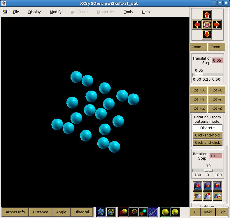
    mixing_beta = 0.7

conv_thr =         1.0d-8
 /

There are several matrix diagonalization options available; Davidson (david) is default and
is fast, ‘cg’ is conjugate gradient-like and slower but uses less memory. Mixing parameters and
conv_thr affect the rate of convergence as one might expect. There are several options in particular
for the nature of the mixing, the user is encouraged to experiment with these, paying close attention to
numerical accuracy. If performing molecular dynamics, these namelists are accompanied by &IONS
and &CELL, please consult the reference at the end of this section for further information on these
and all namelists.

After all the namelists have been specified, a number of other fields are necessary in order to describe
constituent atoms and positions, eg.,

ATOMIC_SPECIES
 Si 28.086 Si.pz-vbc.UPF
ATOMIC_POSITIONS
 Si 0.00 0.00 0.00
 Si 0.25 0.25 0.25

The first section must give atomic label, mass, and the name of the pseudopotential to be used in the
calculation, one line per unique atom. This section is directly followed by details of the unit cell, and
finally the k-points within the Brillouin zone must be specified eg.,

K_POINTS
  10
   0.1250000         0.1250000         0.1250000         1.00
   0.1250000         0.1250000         0.3750000         3.00
   0.1250000         0.1250000         0.6250000         3.00
   0.1250000         0.1250000         0.8750000         3.00
   0.1250000         0.3750000         0.3750000         3.00
   0.1250000         0.3750000         0.6250000         6.00
   0.1250000         0.3750000         0.8750000         6.00
   0.1250000         0.6250000         0.6250000         3.00
   0.3750000         0.3750000         0.3750000         1.00
   0.3750000         0.3750000         0.6250000         3.00

There are a number of ways to specify this data, here the default is used which gives x/y/z and
weight in column four. Additionally, there is a gui utility xcrysden which provides a useful aid in
examining input (as well as output) structure, by loading pw.x files; figure 2 contains a screenshot
for the silicon example given here, and available as example01 in the quantum espresso examples
directory.

Figure 2: screenshot of silicon in xcrysden

Online Reference for px.x :
http://www.quantum-espresso.org/input-syntax/INPUT_PW.html

The following resource has many useful structures.

American Mineralogist Database :
http://rruff.geo.arizona.edu/AMS/amcsd.php

Final Step(s)
There are many useful post-processing options available, including :

   ●   Plotting
   ●   Band structure
   ●   Density of States
   ●   Wannier Functions
   ●   Normal Phonon modes
   ●   NMR parameters

Summary
   ● Select or create Pseudopotentials for constituent atoms
         ○ If creating new files, use ld1.x tool, test rigorously against various AE configurations
             using the &test namelist
         ○ Test using a simple system
   ● Create an input file for the target system; write by hand or use pwgui
         ○ Remember to use one OR other convention for symmetry, pay close attention to units
         ○ Must specify k-points, pseudopotentials and atomic species with positions in unit cell
   ● Post-process if desired
   ●

References
“Pseudopotentials that work: From H to Pu”, G.B.Bachelet, D.R.Hamann, M.Schluter, Phys Rev B,
4199-4228, 26(8), 1982
“Projector augmented wave method”, P. Blochl, Phys Rev B , 17953-17979, 50(24), 1994
“Efficient pseudopotentials for plane-wave calculations”, N.Troullier, J.L.Martins, Phys Rev B, 1993-
2006, 43(3), 1991
“Soft Self-Consistent Pseudopotentials in a Generalized Eigenvalue Formalism”, D.Vanderbilt, Phys
Rev B, 41, 7892, 1991