Quantum integration of elementary particle processes - arXiv
←
→
Page content transcription
If your browser does not render page correctly, please read the page content below
FR-PHENO-2022-01

                                                                           Quantum integration
                                                                     of elementary particle processes
arXiv:2201.01547v2 [hep-ph] 9 Jun 2022

                                                 Gabriele Agliardi1,2 ∗, Michele Grossi3 †, Mathieu Pellen4 ‡, Enrico Prati5,6 §

                                                                          1
                                                                            Dipartimento di Fisica, Politecnico di Milano,
                                                                        Piazza Leonardo da Vinci 32, I–20133 Milano, Italy
                                                                                        2
                                                                                          IBM Italia S.p.A.,
                                                                     Via Circonvallazione Idroscalo, I–20090 Segrate (MI), Italy
                                                            3
                                                                CERN, 1 Esplanade des Particules, Geneva CH–1211, Switzerland
                                                                 4
                                                                     Albert-Ludwigs-Universität Freiburg, Physikalisches Institut,
                                                                      Hermann-Herder-Straße 3, D–79104 Freiburg, Germany
                                                       5
                                                           Istituto di Fotonica e Nanotecnologie, Consiglio Nazionale delle Ricerche,
                                                                      Piazza Leonardo da Vinci 32, I–20133 Milano, Italy
                                                       6
                                                           Dipartimento di Fisica Aldo Pontremoli, Università degli Studi di Milano,
                                                                             Via Celoria 16, Milan, I–20133, Italy

                                                                                             Abstract

                                                 We apply quantum integration to elementary particle-physics processes. In particular,
                                             we look at scattering processes such as e+ e− → q q̄ and e+ e− → q q̄ 0 W. The corresponding
                                             probability distributions can be first appropriately loaded on a quantum computer using
                                             either quantum Generative Adversarial Networks or an exact method. The distributions
                                             are then integrated using the method of Quantum Amplitude Estimation which shows a
                                             quadratic speed-up with respect to classical techniques. In simulations of noiseless quantum
                                             computers, we obtain per-cent accurate results for one- and two-dimensional integration with
                                             up to six qubits. This work paves the way towards taking advantage of quantum algorithms
                                             for the integration of high-energy processes.

                                         ∗
                                           E-mail:   gabrielefrancesco.agliardi@polimi.it
                                         †
                                           E-mail:   michele.grossi@cern.ch
                                         ‡
                                           E-mail:   mathieu.pellen@physik.uni-freiburg.de
                                         §
                                           E-mail:   enrico.prati@unimi.it
Contents
1 Introduction 2
2 Method and tools 3
3 Definition of probability distributions 6
4 Integration of probability distributions 9
5 Conclusion and outlook 15
11 Introduction
In this work, the quantum versions of Monte Carlo algorithms are applied to the problem of
integrating elementary-particle cross sections.
In particle physics, integration methods and Monte Carlo programs play a very special role
as they are the central link between theory and experiment. On the one hand, they allow the
encoding of theoretical predictions including higher-order or beyond-the-Standard-Model effects.
On the other hand, by generating theoretical events according to the underlying distribution,
they allow a one-to-one correspondence with experimental events. Hence theoretical predictions
can be directly compared to experimental measurements in order to get insight into elementary
interactions.
For collider experiments such as the Large Hadron Collider (LHC), Monte Carlo simulations
are crucial as they simulate all the scattering processes generated in the experiment. It means
that considerable computing resources are needed and they are expected to increase further [1, 2].
For some analysis, the limited Monte Carlo statistics is even becoming a significant source of
uncertainty [3, 4]. This calls for a continuous improvement of the performance of such Monte
Carlo generators.
It appears therefore particularly timely to apply quantum versions of Monte Carlo algorithms
to this problem, given the promising advancements in the industry of quantum devices. The core
algorithm of interest for us is Quantum Amplitude Estimation (QAE) [5–8], that was proven to
provide a speedup for the integration of probability distributions, by scaling as O (1/M ), where
√
M is the number of (quantum) samples, as opposed to classical integrators scaling as O(1/ M )
with M (classical) samples. In the context of high-energy physics, this would translate into a
gain in simulation performance, similarly to what was already assessed in other application fields,
and specifically in finance [9–12].
To apply these techniques, classical data must be loaded into a quantum computer, which
is a nontrivial task in terms of computational cost. More precisely, the quantum states that
correspond to the data have to be prepared. In order to encode the data, several algorithms and
techniques are used in the literature [13–18, 10].
While the present work is the first application of QAE algorithms to integration, there have
been numerous applications of quantum computing to other aspects of collider physics. Such
applications have been mainly experiment-oriented: pixel images [19], event topologies [20], event
classification [21], Higgs analysis [22], background suppression [23], measurement unfolding [24] or
jet clustering [25]. Applications to parton-distribution functions (PDF) have also been carried out
by several groups [26, 27] in a quantum context. In addition, several investigations of quantum
parton shower as well as matrix elements evaluation [28, 29] have been carried out [30, 28, 31].
Finally, in Ref. [32] quantum Generative Adversarial Networks (qGAN) [10] techniques have been
used for the purpose of data augmentation.
Here, we focus on two representative cases (e+ e− → q q̄ and e+ e− → q q̄ 0 W processes) to
illustrate the application of QAE. A particularly important point is that the functions to be
integrated are significantly more complicated to than usual Gaussian or log-normal distributions.
These are typically made of trigonometric functions, polynomials, and logarithms (at least for
what concerns the lowest order in perturbative theory). We therefore explore two methods to
prepare the quantum states according to the underlying distribution, namely the qGAN [10] and
an exact loading [33], respectively. Of particular interest for this application, is the ability to
provide correct results when restricting the domain of integration. Finally, we carry out one-
and two-dimensional integration of cross sections. For the latter case, we devise a method that is
2extendable to n dimensions while still allowing the arbitrary reduction of the integration domain.
In general, the integrations are accurate at the per-cent level with up to six qubits.
The article is organised as follows: in the first part, the method and tools used for this work
are presented. The second part deals with two methods to load the probability distributions. The
third one focuses on integrating such probability distributions with quantum amplitude estimate
methods. Finally, the last sections contains a brief summary as well as some concluding remarks.
2 Method and tools
In this section, we first recall some general considerations about Monte Carlo integration and
explain how we translate it to our problem. Second, we briefly describe the processes under
investigation. Finally, the tools used in the next Sections are presented as well as the numerical
input of the cross sections.
General considerations
To start, let us recall some basics of particle physics. A Monte Carlo integration aims at esti-
mating the cross section of scattering processes which can be written schematically as
Z
1
σ= dΦ |M|2 Θ(Φ − Φc ), (1)
F
where F is the flux factor, dΦ the phase-space factor [possibly including parton-distribution
function (PDF)], and |M|2 the matrix element squared which encodes the quantum mechanical
process. In addition, the phase space (also called integration domain below) can be restricted
by the use of so called phase-space cuts which is represented in Eq. (1) by Θ(Φ − Φc ) which we
refer to as the domain function in the following.
In particular, the integration is performed over variables that allow to describe the full phase
space. While these are not physically observable, they allow the full reconstruction of the event
kinematic. In the following, the results are only expressed in terms of these variables that serve as
proxies for physical ones. In particular, the domain restriction (or event selection) is only applied
to the variables of integration. To obtain a physical restriction of the domain of integration, a
simple mapping can be performed. In more general terms, any integral I can be cast into the
following form Z
I= dxf (x)g(x). (2)
The function f describes the probability distribution, while the function g is the integrand
function. In the QAE, f is computed classically, while g is represented by means of a quantum
operator. For example, in Ref. [10], the g function is a linear function which represents the
payoff. In our case, referring to Eq. (1), we take f = |M|2 . We then take g = Θ(Φ − Φc ), so
that g is a generalised Heaviside function which only takes the value 1 or 0; such a function is
sometimes called the indicator function over the integration domain D, and denoted by χD or
1D .1
1
In principle one may also take f = 1 and g = |M|2 Θ(Φ − Φc ), thus eliminating a costly classical pre-
computation. Nonetheless, the implementation complexity on the quantum side rises, and more importantly,
the quantum circuit becomes deeper and wider, meaning that it could not run on currently available quantum
hardware. Consequently we focused our proof of principle on a simplified scenario.
3Classical Core quantum Classical
preprocessing algorithm postprocessing
Distribution Application of
Exact
preparation the domain Integration
distribution
(sampling and filter through through QAE
loading
discretisation) quantum gates
Classical Quantum data Core quantum Classical
preprocessing preparation algorithm postprocessing
Distribution Application of
Distribution
preparation the domain Integration
qGAN training loading
(sampling and filter through through QAE
through qGAN
discretisation) quantum gates
Figure 1: Graphical representation of the two approaches followed in this work. The upper one
uses an exact loading method while the lower one is based on the qGAN.
Implementing this procedure on a quantum computer involves in general two main steps: the
definition of the quantum states and the integration of the probability distribution. The two
approaches that we follow in this work are graphically represented in Fig. 1. The first one is
based on an exact loading while the second relies on the qGAN to prepare the quantum states.
The details of the implementations are explained in the relevant Sections below.
Particle processes investigated
In order to test our numerical approach with the quantum simulations, we have focused on two
simple though non-trivial scattering processes e+ e− → q q̄ and e+ e− → q q̄ 0 W. In particular,
we have not considered hadronic processes as these would require the use of parton distribution
functions.
The first process is e+ e− → q q̄. In quantum electrodynamics (QED), this process is rather
simple. By parametrising the phase space with two angles, the cross section reads:
Z 1 Z 2π
d cos θdφ 1 + cos2 θ .
σ∼ (3)
−1 0
This means that computing such a process (up to an overall normalisation factor) simply amounts
to integrate the function 1 + x2 on the integration domain [−1; 1] while there is no dependence
on φ.
The second one is e+ e− → q q̄ 0 W. In this case, we have considered the full electroweak
Standard Model and not only QED. Due to the three particles in the final state, this process has
5 variables of integration. These can be chosen as two invariants and three angles and the cross
section becomes [34]
4Integral Number of
Process number Description
definition integration variables
Process 1 e+ e− → q q̄ Eq. (3) 2
Process 2 e+ e− → q q̄ 0 W Eq. (4) 5
Table 1: Summary of the elementary processes under investigation.
Z s Z sMax
1
Z 1 Z 2π Z 2π
2
σ∼ dΦ3 Me+ e− →qq̄0 W , (4)
2
MW 0 −1 0 0
with sMax
1 = (s2 − MW ) (s − s2 ) /s2 and dΦ3 = ds2 ds1 d cos θ1 dφ1 dφ2 . As in the previous case,
one of the φ angle is a trivial integration. The main characteristics of the process are summarised
in Table 1.
Software
To check our results, we resorted to an in-house Monte Carlo program, that was used for the
computation of various high-energy physics processes before [35–38]. It is based on the MONACO
integration routine which is a modified version of VEGAS [39] which is part of the VBFNLO
program [40–42]. For the matrix elements, we use either analytical expressions or the matrix-
element generator Recola [43, 44].
Instead, the results in this article are obtained from the open-source distribution Qiskit
[45] which is written in Python. Starting from its libraries, we developed our code to load
events, build probability distributions, and calculating integrals. The specific functions used
are described below in the relevant Sections. With Qiskit, the IBM Quantum Services offer
the possibility to run algorithms on simulated quantum computer as well as test some specific
configurations on real quantum chips.
Input parameters
In order to ease reproduction of our results, we provide below the numerical inputs of our
√
simulations. For the centre-of-mass energy, we have used s = 500 GeV. The electromagnetic
coupling is defined with the help of the Gµ scheme [46] which leads to
√ 2
2 MW
α= 2
Gµ MW 1 − with Gµ = 1.16638 × 10⁻⁵ GeV−2 . (5)
π MZ2
The masses and widths of the massive particles are chosen as [47]
MZOS = 91.1876 GeV, ΓOS
Z = 2.4952 GeV,
OS
MW = 80.379 GeV, ΓOS
W = 2.085 GeV,
(6)
All other fermions are considered massless. The pole masses and widths of the heavy gauge
bosons are determined from the measured on-shell (OS) values [48] via
MVOS ΓOS
V
MV = q , ΓV = q . (7)
1 + (ΓOS
V /M OS )2
V 1 + (ΓV /MVOS )2
OS
53 Definition of probability distributions
A necessary step that enables the usage and exploitation of a quantum algorithm, is the encoding
of data into quantum states, by means of a quantum circuit. Today, it is not possible to rely on
any quantum native techniques like QRAM [49]. Hence, to solve this potential bottleneck, several
approaches were proposed in the literature that allow to encode classical data into quantum states
[50]. This is particularly important as the approximation introduced in data loading could affect
the quality of the integration. This procedure corresponds to the first steps depicted in Fig. 1.
To investigate it, we have classically generated samples (here 10, 000 events) to be loaded
into the quantum state. In particular, we have used two methods: qGAN [10] and an exact
loading [33], respectively. Both approaches will be outlined and compared in the following. In
+ −
this
R +1 Section, we2
focus on the simple case of e e → q q̄ in QED which 2.
amounts to integrate
−1 dx 1 + x , meaning that the distribution to be loaded is 1 + x
We discuss first the qGAN method for our application. A Generative Adversarial Network
(GAN) [51], in its classical form, is characterised by the interplay of a generative network and
a discriminative network to learn the probability distribution underlying the training data [52].
A qGAN has a similar structure, but the generator is a parametrised quantum circuit (PQC)
instead of a classical neural network. This way the generator is trained to load a quantum state,
approximating the discretised version of the target distribution. As a consequence, this algorithm
belongs to the general class of quantum variational algorithms, namely hybrid algorithms that
rely on a continuous interaction between a quantum computer and a classical computer. An
initial PQC is defined (called ansatz ) and then using a classical optimiser this circuit is trained
iteratively. The update of the parameters is driven by the evolution of the related loss function.
There are no general prescriptions about the structure of the variational circuit, so that challenges
remain, including the trainability, accuracy and efficiency of any variational quantum circuits.
For a general overview of variational algorithms, we refer the reader to Ref. [53].
To apply such a method to the integration of the e+ e− → q q̄ cross section, weRhave loaded the
+1
normalised distribution 1 + x2 , which we define as p(x) = (1 + x2 ) 83 such that −1 dxp(x) = 1,
using the implementation of the qGAN in Qiskit [10].2 The results obtained are presented in
Fig. 2 and Table 2 where several loaded distributions are compared against the true value of
the distribution for two cases. The first one is the default loading obtained from default qGAN
parameters defined in Qiskit, while the second one is an optimised version of the neural network
for this particular functional form obtained after several tests of different variational forms and
optimiser parameters.
In both cases, five random seeds have been used to estimate the spread of the loading pro-
cedure. From this example, it should be rather clear that an optimisation of the neural network
in terms of architecture (rotation gates and entanglement gates) as well as parameters tuning is
needed and that a default configuration cannot be used for arbitrary distributions. Specifically,
from our study, the best entanglement is the circular one and the best results are obtained with
a learning rate of 5.10−4 and 1.10−3 for the generator and discriminator, respectively.3 The
improvement in the accuracy of the loading can be observed in Fig. 2 and Table 2. Other strate-
gies for the entanglement layers (full, linear, or SCA) give rather unstable results depending on
the seeds used. Increasing the number of repetitions does not appear to improve the loading
accuracy.
2
See for example https://Qiskit.org/documentation/tutorials/finance/10_qgan_option_pricing.html
for the original implementation of Ref. [10].
3
The default values of the learning rate for the generator and discriminator are 1.10−3 and 1.10−5 , respectively.
6Difference per bin [%]
qGAN loading σx
Min. Max. Average
Default 1 +3.46 −25.1 14.6 0.0206
Default 2 +3.90 +19.3 12.0 0.0152
Default 3 +2.36 −21.1 8.51 0.0118
Default 4 +1.48 −40.2 13.7 0.0230
Default 5 +0.224 −31.7 12.0 0.0171
Optimised 1 −0.351 −10.0 4.70 7.13 × 10⁻³
Optimised 2 −0.811 −18.1 7.69 0.0121
Optimised 3 −0.052 −10.1 4.92 7.83 × 10⁻³
Optimised 4 +0.599 −15.4 5.16 7.64 × 10⁻³
Optimised 5 −0.995 −12.4 4.65 7.00 × 10⁻³
Table 2: Comparison of qGAN loading of the normalised 1 + x2 distribution for the default
learning rates and an optimised one. The results are given for 5 different seeds. The minimum,
maximum, and average difference per bin with respect to the true value is provided (in per cent).
The root mean squared error from the true value is also given.
In our example, the default qGAN can lead to loading errors up to 40% with an average
deviation above 10% per bin. In the case of an optimised neural network, the average accuracy
of the loading per bin is significantly better and lies around 5%. To measure the quality of the
whole loaded distribution, one can revert to the root mean squared error defined as
v
u
u1 X N
σx = t (xi − µi )2 , (8)
N
i=1
where i denotes the bins, xi the value of the distributions loaded, and µi the true value of the
distribution.
Finally, the better behaviour of the tuned qGAN can be also observed in the relative entropy
as a function of the time steps in Fig. 2. The relative entropy S is defined as
N −1
X P (x)
S= P (x) log , (9)
Q(x)
x=0
where P and Q are the output distribution of the quantum generator and the discretised version
of the target distribution, respectively. The tuned network shows a much smoother converge
than the default one.
We now turn to the exact loading which is represented in Fig. 3. Such a technique is an
analytical way to initialise complex amplitude on qubit register. Being an exact method, the
accuracy of the loaded distribution is obviously better than with the qGAN. This is shown
quantitatively in Table 3 where the differences per bin are shown for the best bin, the worst, and
the average. For the two qGAN cases above, the best seed has been selected. From Table 3, it is
rather clear that the exact loading is performing significantly better in this case. In particular,
it shows discrepancies from the truth by no more than 2% and is on average around 1%. This
order of magnitude should be kept in mind as the best possible loading accuracy with a sample
of 10, 000 events.
7Relative Entropy Relative Entropy
0.8 1.0
0.7
0.8
0.6
relative entropy seed 5
relative entropy seed 5
0.5 0.6
0.4
0.3 0.4
0.2
0.2
0.1
0.0 0.0
0 200 400 600 800 1000 0 200 400 600 800 1000
time steps time steps
Distribution Distribution
(1+x^2)*3/8 (1+x^2)*3/8
0.175 simulation seed 1 0.175 simulation seed 1
simulation seed 2 simulation seed 2
0.150 simulation seed 3 0.150 simulation seed 3
simulation seed 4 simulation seed 4
simulation seed 5 simulation seed 5
0.125 0.125
0.100 0.100
p(x)
p(x)
0.075 0.075
0.050 0.050
0.025 0.025
0.000 0.000
0.875 0.125 1.125 0.875 0.125 1.125
x x
Figure 2: Loading with qGAN of the normalised 1 + x2 distribution with the default learning
rate (left) and an optimised one (right). In both cases, it is compared to the compared to the
theoretical value (thick orange curve) and the entanglement is circular.
Distribution
(1+x^2)*3/8
0.175 simulation
0.150
0.125
0.100
p(x)
0.075
0.050
0.025
0.000
0.875 0.125 1.125
x
Figure 3: Direct loading of the the normalised 1 + x2 distribution (blue histogram) compared to
the theoretical value (orange curve).
8Difference per bin [%]
Loading σx
Min. Max. Average
Direct +0.207 −1.88 1.35 1.80 × 10⁻³
qGAN default +2.36 −21.1 8.51 0.0118
qGAN optimised −0.995 −12.4 4.65 7.00 × 10⁻³
Table 3: Comparison of qGAN loading of the normalised 1 + x2 distribution for the default
learning rates and an optimised one as well as the direct loading. The qGAN results are the
ones of the best seed in table 2. The minimum, maximum, and average difference per bin with
respect to the true value is provided (in per cent). The root mean squared error from the true
value is also given.
If instead, one loads the exact distribution which is known analytically (as opposed to a
sample generated according to it), there is simply no deviation from the true distribution. This
aspect is particularly important as in principle, a closed form of the distribution is not necessarily
available. It also means that the quality of the exact loading is directly dependent on the statistics
of the sample given as input.
In order to represent the target distributions with N bins, one needs to encode a statevector of
size N , and this translates into a number of qubits n such that N = 2n . In other words, the data
resolution is a direct consequence of the number of qubits used. Obviously, the computational
complexity is related to such n, as well. As far as the qGAN approach is concerned, and discarding
the training process that will be discussed in the next paragraph, the pure loading phase requires
O(poly(kn)) gates, where k is the number of layers, which is intrisic in the definition of the ansatz.
Assuming that k can be kept under control, qGANs become an efficient data loading technique,
and preserve the speedup of the Quantum Amplitude Estimation algorithm for integration [10].
Conversely, for the exact loading algorithm, the number of 2-qubit gates scales as O(2n ) [33].
In the argument above, the training cost of a qGAN is neglected. This is motivated by the fact
that the same distribution is typically used for multiple simulations, and in this case the training
process is performed once, so that the training time can be seen as a constant. Nonetheless,
it is worth saying that the scaling of the training cost when the distribution size grows, is an
open question, whose complexity lies in the unpredictable number of epochs needed to achieve
training convergence, in the desired level of approximation, and in the different behavior of
various optimisers. The interaction of such hyperparameters on small-scale problems is discussed
in Ref. [54].
Given the limited amount of qubits in our study, we could not appreciate the benefits of
qGANs in terms of scaling, while on the contrary we had to face the learning, possibly the tun-
ing of the network, and the verification of the result. Moreover, the current absence of analytical
estimates for approximations induced by qGANs, limits their applicability for computing arbi-
trary processes in a quantum Monte Carlo program, especially when probability distributions
are known from first principle or vast amounts of classical data representing them are available.
4 Integration of probability distributions
In this section, we exclusively discuss the integration of probability distributions. While we could
also use the qGAN loading, we use exclusively the exact loading method in this Section in order
to isolate the integration step from the loading one. In particular, we look at the integration of
9one- and two-dimensional distributions. This procedure corresponds to the core of the work flow
depicted in Fig. 1.
Once the target distribution has been loaded into a quantum channel, the integration is
performed through QAE. Assuming efficient data loading, the algorithm achieves a quadratic
improvement, compared with classical Monte Carlo simulation. QAE is a very interesting and
studied quantum algorithm due to its potential application in different fields such as quantum
chemistry, machine learning, finance and high energy physics. QAE is a fundamental routine in
quantum computing which generalises the idea behind the Grover’s search algorithm, and gives
rise to a family of quantum algorithms. The basic idea is that given an operator A that acts as
√ √
A|0i = 1 − a|Ψ0 i + a|Ψ1 i (10)
where a ∈ [0, 1] and |Ψ0 i and |exΨ1 i are two normalised states. Quantum Amplitude Estimation
(QAE) is the task of finding an estimate for the amplitude a of the state |Ψ1 i:
a = |hΨ1 |Ψ1 i|2 .
This can be achieved by the definition of a Grover’s like operator of the form [5]:
Q = AS0 A† SΨ1 , (11)
where S0 and SΨ1 are reflections about the |0i and |Ψ1 i states, respectively, and phase estimation.
This formulation represents the canonical version of QAE which is a combination of Quantum
Phase Estimation (QPE) and Grover’s Algorithm [55]. On one hand, QPE is theoretically able to
achieve exponential speedup, like in the famous Shor’s Algorithm for factoring [56], on the other
hand its practical implementation in terms of qubits and circuit depth represents an interesting
challenge in current technological scenario. Removing the dependence on QPE for a QAE-like
routine in a simplified version such that it uses only Grover iterations has been largely studied
in the literature.
Indeed, there exist different implementations, with respect to the original QAE implemen-
tation by Brassard et al. [5], such as the Iterative Amplitude Estimation (IAE) version which
does not rely on Quantum Phase Estimation (QPE) as defined in Eq.(11). This is the adopted
version for this work which can achieve a provable quadratic speedup over classical Monte Carlo
simulation, with a desired asymptotic behaviour in its iterative queries to the quantum com-
puter, reducing the required number of qubits and gates [6]. Additional implementations are the
Maximum Likelihood Amplitude Estimation [7, 8] which limit resorting to expensive controlled
operations.
One-dimensional distribution
As mentioned in the previous section, the direct loading adds no approximation to the probabili-
ties given as input. If such probabilities are obtained through sampling, though, they are in turn
approximated. This means eventually that the result of the integration will strongly depend on
the quality of the input. To illustrate this, we have use the QAE with samples of different sizes:
1000 events (low statistics), 100,000 events (high statistics), 1M events (very high statistics). In
particular, we have made used of the Qiskit functions LinearAmplitudeFunction [15, 16],
EstimationProblem, and IterativeAmplitudeEstimation. The latter implement and im-
proved version of the original QAE method [6]. The results for the different samples and the
loading of the exact distribution are compared to the analytical result in Tables 4 and 5. In
10low stat. high stat. very high stat. exact
Domain
σ δ[%] σ δ[%] σ δ[%] σ δ[%]
[−0.75; 0.75] 0.664 0.592 0.664 0.622 0.668 0.0280 0.668 −2.01 × 10⁻³
[−0.5; 0.5] 0.403 0.794 0.402 1.16 0.406 0.122 0.406 −6.01 × 10⁻³
[−0.25; 0.25] 0.196 −2.42 0.189 1.01 0.192 −0.166 0.191 −0.0175
Table 4: Symmetric integration of the normalised 1+x2 probability distribution based on samples
with different statistics (low, high, and very high) or the exact probability distribution. The
results are compared to the analytical result in per cent. The results are obtained for three
qubits. The low, high, and very high statistics refer to 10, 000, 100, 000, and 1 million events,
respectively.
low stat. high stat. very high stat. exact
Domain
σ δ[%] σ δ[%] σ δ[%] σ δ[%]
[−0.75; 0] 0.345 −3.31 0.332 0.706 0.334 0.0331 0.334 −8.31 × 10⁻³
[−0.5; 0] 0.215 −5.86 0.201 1.15 0.203 0.0986 0.203 −0.0161
[−0.25; 0] 0.112 −17.1 0.0939 1.87 0.0960 −0.284 0.0957 −0.0389
Table 5: Asymmetric integration of the normalised 1 + x2 probability distribution based on
samples with different statistics (low, high, and very high) or the exact probability distribution.
The results are compared to the analytical result in per cent. The results are obtained for three
qubits. The low, high, and very high statistics refer to 10, 000, 100, 000, and 1 million events,
respectively.
these Tables and the following ones, δ[%] = σ−σ σtruth in per cent, where σtruth denotes the true
truth
analytical integration.
It is particularly visible that the quality of the integration is dependent on the statistics
used. For 1 million events, the result of the integration is accurate at around the per-mille
level. The loading of the exact distribution, on the other hand, is systematically below half
a per mille accuracy. In addition, it is worth emphasising that the relevant statistics for the
integration precision is not the one of the full sample but of the sample in the integrated region.
This is particularly clear in Tables 4 and 5 where the smaller integration domain have a lower
accuracy. This holds true also for the the loading of the exact distribution. It is worth noticing
that the relative differences with respect to the true values in Tables 4 and 5 do not necessarily
display a scaling behaviour according to the statistics. This is due to the fact that the samples
are subject to statistical fluctuation and their central value (as opposed to the error) follow a
scaling behaviour only on average and not for every single point. These numbers are particularly
useful as they provide an estimate of the error which originates from not knowing the original
distribution analytically (as in the 2D case below). In the present case, this error is about few
per cent.
While in Tables 4 and 5, the limits of integration corresponds to the eight bins (n = 3 qubits
give 2n bins) on the domain [−1; 1], in Tables 6 and 7 the same exercise is performed with this
time integration domains that do not fit the binning of the piecewise definition of the function.
In the present case, only the results of the integration of the high-statistics sample as well as
the exact result are provided as a function of the number of qubits. In general, one observes that
the results are significantly worse than in the previous case. This is simply due to the ill-defined
11[−0.7; 0.7] [−0.625; 0.625]
Qubits number high stat. exact high stat. exact
σ δ[%] σ δ[%] σ δ[%] σ δ[%]
3 0.402 −34.3 0.406 −33.5 0.402 −24.2 0.406 −23.3
4 0.525 −14.1 0.530 −13.2 0.525 −0.933 0.530 3.67 × 10⁻³
5 0.592 −3.05 0.597 −2.27 0.525 −0.933 0.530 3.67 × 10⁻³
6 0.592 −3.05 0.597 −2.27 0.525 −0.933 0.530 3.67 × 10⁻³
Table 6: Symmetric integration of the normalised 1 + x2 probability distribution based on a 1
million-events samples as well as the exact probability distribution. The results are compared to
the analytical result in per cent as a function of the number of qubits. The high statistics refer
to 100, 000 events.
[−0.7; 0.6] [−0.625; 0.375]
Qubits number high stat. exact high stat. exact
σ δ[%] σ δ[%] σ δ[%] σ δ[%]
3 0.402 −28.0 0.406 −27.1 0.296 −28.1 0.299 −27.5
4 0.463 −17.0 0.468 −16.0 0.408 −1.07 0.412 5.96 × 10⁻³
5 0.527 −5.46 0.532 −4.62 0.408 −1.07 0.412 5.96 × 10⁻³
6 0.542 −2.76 0.547 −1.81 0.408 −1.07 0.412 5.96 × 10⁻³
Table 7: Asymmetric integration of the normalised 1 + x2 probability distribution based on a 1
million-events samples as well as the exact probability distribution. The results are compared to
the analytical result in per cent as a function of the number of qubits. The high statistics refer
to 100, 000 events.
value of the distribution between two bins. By increasing the number of qubits, one observes an
improvement of the results until the bin edges correspond to the integration boundaries. Once
the bin edges fit the integration boundaries, increasing the number of qubits does not lead to
any improvement as the distribution is already best defined within the integration boundaries.
This implies that when taking the limit of large numbers of qubits, these artifacts disappear.
Two-dimensional distribution
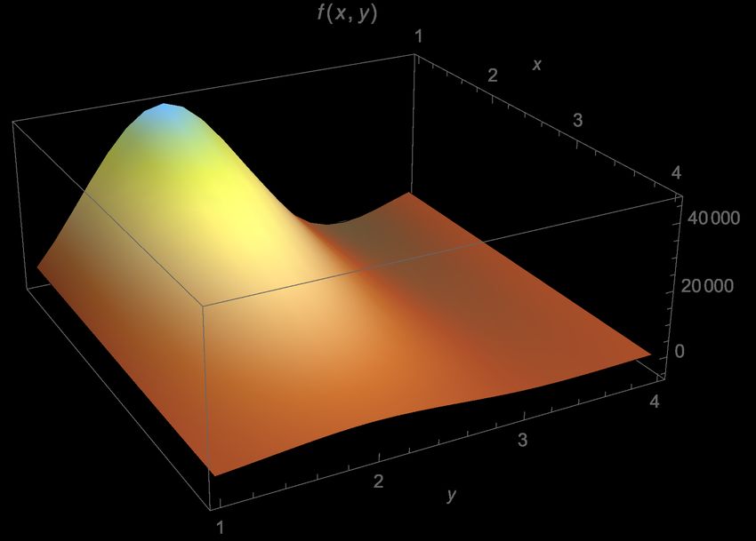
We now turn to the integration of a two-dimensional function for the case of e+ e− → q q̄ 0 W. As
it can be seen from Eq. (4), the 3-particles phase space requires the integration over 5 variables.
To simplify the problem while keeping it non-trivial, we integrate over the two invariants s1 and
s2 . To that end, we take a slice in Eq. (4) by setting cos θ1 = 0, φ1 = π/2, and φ2 = π/2. The
cross section then becomes
Z s Z sMax
1
2
σ∼ dΦ̃3 M0 , (12)
2
MW 0
with dΦ̃3 = ds2 ds1 and M0 = Me+ e− →qq̄0 W (cos θ1 = 0, φ1 = π/2, φ2 = π/2). The integration
of the cross section therefore amounts to integrate over the variables s2 and s1 . The integrand
is graphically represented on the left-hand side of Fig. 4 as a function of x = s2 and y = s1 .
Again, we would like to stress that, as in the one-dimensional case, the type of functions to be
12y
0 x
Figure 4: Two-dimensional numerical representation of the integrand in Eq. (12) with x = s2
and y = s1 (left). Graphical representation of the mapping of the two-dimensional function to a
one dimensional function (right). The blue shaded area represents a restriction of the domain of
integration.
integrated are rather different and more complicated than those that have been tested so far
such as Gaussian or log-normal distributions.
To encode the multidimensional distribution of Eq. (12) on qubits register, we revert to the
same method as in the one-dimensional case by defining it piecewise. To that end, we introduce
a mapping from the two dimensional function to one-dimensional. The way the mapping is
performed is represented in the right-hand side of Fig. 4. We opt for this solution instead of
simply scanning from left to right and top to bottom, in order to ensure that any physically
motivated integration domain restrictions can be mapped to the one-dimensional function in
a continuous way, hence minimising the error due to interpolations that are not evident nor
considered in previous one-dimensional case. We note that this method is fully general and can
be extended to n-dimensional integral. It has also the advantage to be fully flexible and allow
for the arbitrary phase-space cut in the integrand. For example in Fig. 4, the blue shaded area
represents the restriction of the integration domain. In this case, assuming that the first bin of
the 1D function [f˜ 7→ f˜(X)] is in the top left corner and that it is mapped to SX = [0; 16], break
points will be introduced at X = 6, X = 10, X = 14, and X = 15.
For the present experiment, we have produced 100, 000 events according to the two-dimensional
distribution over the full integration domain. We reduced the latter by setting the maximum
value of s2 to 20, 000 in order to avoid populating bins with very few events. This leads to a
total of 97, 581 events.
The results of our experiments are given in Table 8. In this case, we consider two cases of
integrand reduction or cuts: S1 which implement the cut [62, 500; 187, 500] × [5, 000; 10, 000] and
S2 which corresponds to [80, 000; 150, 000] × [5, 000; 10, 000]. The main difference between these
two sub-domains is that the boundaries of S1 fits the edges of the bins of a 4 × 4 grid while the
ones of S2 do not for the first variable.
This explains why in Table 8 for the 4 × 4 grid, the result of the integration is perfectly
13Qubits S1 S2
Grid dim.
number σ δ[%] σ δ[%]
4 4×4 0.55 0 0.70 −4.1
5 5×5 0.52 −4.92 0.53 −26.6
6 6×6 0.47 −14.1 0.79 9
6 7×7 0.62 −14.4 0.70 −3.0
6 8×8 0.55 0 0.78 7.6
Table 8: Two-dimensional integration with two different integration domains: one which matches
bin edges (S1 ) and the other does not (S2 ). The numerical integrations are compared to the value
obtained from the classical sample for different grid dimensions corresponding to different number
of qubits. .
reproducing the truth (σ = 0.545833717629457) which is here the classical sample. While in the
one-dimensional case, each increase in the number of qubits translates into the halving of the
bins, it is not the case here. Indeed, going from 4 qubits to 5, only allows to extend the grid
from 4 × 4 to 5 × 5. It explains why for S1 , while increasing the grid and making the binning
finner, the accuracy of the integration does not improve. It only becomes perfect again when the
binning is again perfectly fitting the boundaries of the integration domain.
This is further exemplified with the case of S2 where the improvement is not uniform
when increasing the grid dimension. For this case, the true value of the cross section is σ =
0.7244852993923. This is due, on the one hand, to the fact that the edges of the second dimen-
sion are only matched for the cases of the 4 × 4 and 8 × 8 grids. On the other hand, as seen in the
one dimensional case, when the domain of integration does not match the piecewise definition of
the function, the result of the integration is uncontrolled. In the present case, the interpolation
is such that doubling the number of bins in each dimension does not necessarily increase the
precision of the integration (grid 4 × 4 vs. grid 8 × 8).
This implies that only a large number of qubits (implying finer bins) can allow a reliable
estimate of the integral. In particular, for the present application which the computation of
cross sections in collider experiments, the usual standard for Monte Carlo error is to reach a per
mille accuracy. With current technology, this goal could be challenging. Nonetheless, we believe
that with the advent of machines with 1000 qubits or more4 , this is perfectly conceivable. Not
only a greater number of qubits is needed but also a greater quantum volume [57] that could
allow to run QAE on a quantum computer, where further improvements are required, e.g., longer
coherence times and higher gate fidelity.
We note in passing that with our method, we could in principle also sample events according
to the underlying distribution as done in Ref. [32]. We defer the study of this aspect to future
work. In particular, while the integration of probability distributions with QAE methods has
shown to provide a quantum advantage, it is not clear yet if such an advantage can also be
observed for the sampling of events.
4
See for example, IBM recent Roadmap to Scaling Quantum Technology announcing aiming at 1000-plus qubits
by 2023.
145 Conclusion and outlook
This work constitutes the first application of Quantum Amplitude Estimate (QAE) algorithm to
high-energy physics. To test its feasibility we have checked two non-trivial elementary processes,
namely e+ e− → q q̄ and e+ e− → q q̄ 0 W.
Complex function appearing in elementary scattering processes can successfully be loaded
onto qubits consistently with the results of Ref. [32]. To load the functions we have used two
methods, namely: the quantum Generative Adversarial Networks (qGAN) [10] and an exact
loading [33]. For our purposes, we have found that the latter one is more appropriate due to
its versatility and reliability for what concerns application with a small number of qubits. In
particular, it does not require any training nor tuning which makes it very easy to use.
In addition, we have successfully used the QAE algorithm for the integration of the two
elementary processes in one and two dimensions, respectively. In particular, we have tested the
reliability of the integration when restricting its domain of integration, which would correspond
to imposing physical event selection in an experiment. To integrate multi-dimensional functions,
we have devised a general method which can be extended to n dimensions.
Following this purely numerical strategy requires large number of qubits in order to be ac-
curate. For our application, we have found that QAE provides per-cent accurate results for
one- and two-dimensional integration with up to six qubits. The results support the framework
where future physical devices will make quantum computing a viable solution for integrating
elementary processes in high-energy physics. An increase in the number of available qubits is
critical for the practical application to our domain of study. It should be noted here, though,
that other issues emerge in the current era of Noisy Intermediate-Scale Quantum Computers [58].
Indeed, additional challenges originate from the imperfection of present hardware construction,
from the limited topological connectivity of qubits, and from the inability to put in place full
error correction protocols that would require additional qubits and resources. Practical usage
of the algorithms shall therefore be validated and perfected also through the execution on real
quantum devices.
This work opens new perspectives for the computation of particle processes with quantum
Monte Carlo integration techniques. Following the same method, more complicated processes
(with higher multiplicities and hadronic processes) can be investigated.
Acknowledgements
The Authors are grateful to Julien Gacon, Ivano Tavernelli, Sofia Vallecorsa, and Christa Zoufal
for useful discussions. We acknowledge use of the IBM Quantum platform for this work. This
project is supported by CERN Quantum Technology Initiative. The views expressed are those
of the authors and do not reflect the official policy or position of IBM company or the IBM
Quantum team. GA is grateful to IBM for supporting his Executive PhD. GA and EP are
thankful for the access to the IBM Quantum Researchers Program. MP acknowledges support
from the German Research Foundation (DFG) through the Research Training Group RTG2044.
References
[1] A. Buckley, Computational challenges for MC event generation. J. Phys. Conf. Ser. 1525
(2020) no. 1, 012023, arXiv:1908.00167 [hep-ph].
15[2] HSF Physics Event Generator WG Collaboration, S. Amoroso et al., Challenges in
Monte Carlo Event Generator Software for High-Luminosity LHC. Comput. Softw. Big
Sci. 5 (2021) no. 1, 12, arXiv:2004.13687 [hep-ph].
[3] ATLAS Collaboration, G. Aad et al., Search for the electroweak diboson production in
association with a high-mass dijet system in semileptonic final states in pp collisions at
√
s = 13 TeV with the ATLAS detector. Phys. Rev. D 100 (2019) no. 3, 032007,
arXiv:1905.07714 [hep-ex].
[4] CMS Collaboration, A. M. Sirunyan et al., Search for anomalous electroweak production
of vector boson pairs in association with two jets in proton-proton collisions at 13 TeV.
Phys. Lett. B 798 (2019) 134985, arXiv:1905.07445 [hep-ex].
[5] G. Brassard, M. Mosca, and A. Tapp, Quantum Amplitude Amplification and Estimation.
Quantum Computation and Information 305 (2002) , arXiv:quant-ph/0005055
[quant-ph].
[6] D. Grinko, J. Gacon, C. Zoufal, and S. Woerner, Iterative Quantum Amplitude Estimation.
npj Quantum Inf 7 (2021) no. 52, , arXiv:1912.05559 [quant-ph].
[7] Y. Suzuki, S. Uno, R. Raymond, T. Tanaka, T. Onodera, and N. Yamamoto, Amplitude
estimation without phase estimation. Quantum Information Processing 19 (2020) no. 75, ,
arXiv:1904.10246 [quant-ph].
[8] K. Nakaji, Faster Amplitude Estimation. Quantum Information & Computation 2020 20
(2020) no. 13&14, , arXiv:2003.02417 [quant-ph].
[9] P. Rebentrost, B. Gupt, and T. R. Bromley, Quantum computational finance: Monte Carlo
pricing of financial derivatives. Physical Review A 98 (2018) 022321.
[10] C. Zoufal, A. Lucchi, and S. Woerner, Quantum Generative Adversarial Networks for
Learning and Loading Random Distributions. npj Quantum Inf 5 (2019) no. 103, ,
arXiv:1904.00043 [quant-ph].
[11] N. Stamatopoulos, D. J. Egger, Y. Sun, C. Zoufal, R. Iten, N. Shen, and S. Woerner,
Option Pricing using Quantum Computers. Quantum 4 (2020) 291, arXiv:1905.02666.
[12] N. Stamatopoulos, G. Mazzola, S. Woerner, and W. J. Zeng, Towards Quantum Advantage
in Financial Market Risk using Quantum Gradient Algorithms. arXiv:2111.12509
[quant-ph].
[13] L. Grover and T. Rudolph, Creating superpositions that correspond to efficiently integrable
probability distributions. arXiv:quant-ph/0208112 [quant-ph].
[14] A. Adedoyin, J. Ambrosiano, P. Anisimov, A. Bärtschi, W. Casper, G. Chennupati,
C. Coffrin, H. Djidjev, D. Gunter, S. Karra, et al., Quantum algorithm implementations
for beginners. arXiv:1804.03719 [cs.ET].
[15] S. Woerner and D. J. Egger, Quantum risk analysis. npj Quantum Information 5 (2019)
no. 1, 1–8, arXiv:1806.06893 [quant-ph].
16[16] J. Gacon, C. Zoufal, and S. Woerner, “Quantum-enhanced simulation-based optimization,”
in 2020 IEEE International Conference on Quantum Computing and Engineering (QCE),
pp. 47–55, IEEE. 2020. arXiv:2005.10780 [quant-ph].
[17] A. Holmes and A. Matsuura, “Efficient quantum circuits for accurate state preparation of
smooth, differentiable functions,” in 2020 IEEE International Conference on Quantum
Computing and Engineering (QCE), pp. 169–179, IEEE. 2020. arXiv:2005.04351
[quant-ph].
[18] J. J. García-Ripoll, Quantum-inspired algorithms for multivariate analysis: from
interpolation to partial differential equations. Quantum 5 (2021) 431, arXiv:1909.06619
[quant-ph].
[19] S. Y. Chang, S. Herbert, S. Vallecorsa, E. F. Combarro, and R. Duncan,
Dual-Parameterized Quantum Circuit GAN Model in High Energy Physics. EPJ Web
Conf. 251 (2021) 03050, arXiv:2103.15470 [quant-ph].
[20] M. Kim, P. Ko, J.-h. Park, and M. Park, Leveraging Quantum Annealer to identify an
Event-topology at High Energy Colliders. arXiv:2111.07806 [hep-ph].
[21] P. Bargassa, T. Cabos, S. Cavinato, A. Cordeiro Oudot Choi, and T. Hessel, Quantum
algorithm for the classification of supersymmetric top quark events. Phys. Rev. D 104
(2021) no. 9, 096004, arXiv:2106.00051 [quant-ph].
[22] V. Belis, S. González-Castillo, C. Reissel, S. Vallecorsa, E. F. Combarro, G. Dissertori, and
F. Reiter, Higgs analysis with quantum classifiers. EPJ Web Conf. 251 (2021) 03070,
arXiv:2104.07692 [quant-ph].
[23] J. Heredge, C. Hill, L. Hollenberg, and M. Sevior, Quantum Support Vector Machines for
Continuum Suppression in B Meson Decays. arXiv:2103.12257 [quant-ph].
[24] K. Cormier, R. Di Sipio, and P. Wittek, Unfolding measurement distributions via quantum
annealing. JHEP 11 (2019) 128, arXiv:1908.08519 [physics.data-an].
[25] A. Y. Wei, P. Naik, A. W. Harrow, and J. Thaler, Quantum Algorithms for Jet Clustering.
Phys. Rev. D 101 (2020) no. 9, 094015, arXiv:1908.08949 [hep-ph].
[26] A. Pérez-Salinas, J. Cruz-Martinez, A. A. Alhajri, and S. Carrazza, Determining the
proton content with a quantum computer. Phys. Rev. D 103 (2021) no. 3, 034027,
arXiv:2011.13934 [hep-ph].
[27] T. Li, X. Guo, W. K. Lai, X. Liu, E. Wang, H. Xing, D.-B. Zhang, and S.-L. Zhu, Partonic
Structure by Quantum Computing. arXiv:2106.03865 [hep-ph].
[28] K. Bepari, S. Malik, M. Spannowsky, and S. Williams, Towards a quantum computing
algorithm for helicity amplitudes and parton showers. Phys. Rev. D 103 (2021) no. 7,
076020, arXiv:2010.00046 [hep-ph].
[29] S. Ramírez-Uribe, A. E. Rentería-Olivo, G. Rodrigo, G. F. R. Sborlini, and L. Vale Silva,
Quantum algorithm for Feynman loop integrals. arXiv:2105.08703 [hep-ph].
17[30] C. W. Bauer, W. A. de Jong, B. Nachman, and D. Provasoli, Quantum Algorithm for High
Energy Physics Simulations. Phys. Rev. Lett. 126 (2021) no. 6, 062001,
arXiv:1904.03196 [hep-ph].
[31] S. Williams, S. Malik, M. Spannowsky, and K. Bepari, A quantum walk approach to
simulating parton showers. arXiv:2109.13975 [hep-ph].
[32] C. Bravo-Prieto, J. Baglio, M. Cè, A. Francis, D. M. Grabowska, and S. Carrazza,
Style-based quantum generative adversarial networks for Monte Carlo events.
arXiv:2110.06933 [quant-ph].
[33] V. V. Shende, S. S. Bullock, and I. L. Markov, Synthesis of quantum-logic circuits. IEEE
Transactions on Computer-Aided Design of Integrated Circuits and Systems 25 (2006)
no. 6, 1000–1010, arXiv:quant-ph/0406176 [quant-ph].
[34] E. Byckling and K. Kajantie, Particle kinematics.
[35] R. Gavin, C. Hangst, M. Krämer, M. Mühlleitner, M. Pellen, E. Popenda, and M. Spira,
Matching Squark Pair Production at NLO with Parton Showers. JHEP 10 (2013) 187,
arXiv:1305.4061 [hep-ph].
[36] R. Gavin, C. Hangst, M. Krämer, M. Mühlleitner, M. Pellen, E. Popenda, and M. Spira,
Squark Production and Decay matched with Parton Showers at NLO. Eur. Phys. J. C 75
(2015) no. 1, 29, arXiv:1407.7971 [hep-ph].
[37] L. Ali Cavasonza, M. Krämer, and M. Pellen, Electroweak fragmentation functions for dark
matter annihilation. JCAP 02 (2015) 021, arXiv:1409.8226 [hep-ph].
[38] L. Ali Cavasonza, H. Gast, M. Krämer, M. Pellen, and S. Schael, Constraints on
leptophilic dark matter from the AMS-02 experiment. Astrophys. J. 839 (2017) no. 1, 36,
arXiv:1612.06634 [hep-ph]. [Erratum: Astrophys.J. 869, 89 (2018)].
[39] G. P. Lepage, A New Algorithm for Adaptive Multidimensional Integration. J. Comput.
Phys. 27 (1978) 192.
[40] K. Arnold et al., VBFNLO: A Parton level Monte Carlo for processes with electroweak
bosons. Comput. Phys. Commun. 180 (2009) 1661–1670, arXiv:0811.4559 [hep-ph].
[41] J. Baglio et al., VBFNLO: A Parton Level Monte Carlo for Processes with Electroweak
Bosons – Manual for Version 2.7.0. arXiv:1107.4038 [hep-ph].
[42] J. Baglio et al., Release Note - VBFNLO 2.7.0. arXiv:1404.3940 [hep-ph].
[43] S. Actis, A. Denner, L. Hofer, A. Scharf, and S. Uccirati, Recursive generation of one-loop
amplitudes in the Standard Model. JHEP 04 (2013) 037, arXiv:1211.6316 [hep-ph].
[44] S. Actis, A. Denner, L. Hofer, J.-N. Lang, A. Scharf, and S. Uccirati, RECOLA: REcursive
Computation of One-Loop Amplitudes. Comput. Phys. Commun. 214 (2017) 140–173,
arXiv:1605.01090 [hep-ph].
[45] M. Treinish and et al., Qiskit/qiskit: Qiskit 0.33.0, Dec., 2021.
https://doi.org/10.5281/zenodo.5762490.
18[46] A. Denner, S. Dittmaier, M. Roth, and D. Wackeroth, Electroweak radiative corrections to
e+ e− → W W → 4 fermions in double pole approximation: The RACOONWW approach.
Nucl. Phys. B587 (2000) 67–117, arXiv:hep-ph/0006307 [hep-ph].
[47] ParticleDataGroup Collaboration, M. Tanabashi et al., Review of Particle Physics.
Phys. Rev. D98 (2018) no. 3, 030001.
[48] D. Yu. Bardin, A. Leike, T. Riemann, and M. Sachwitz, Energy-dependent width effects in
e+ e− -annihilation near the Z-boson pole. Phys. Lett. B206 (1988) 539–542.
[49] V. Giovannetti, S. Lloyd, and L. Maccone, Quantum Random Access Memory. Phys. Rev.
Lett. 100 (2008) 160501.
[50] M. Schuld, R. Sweke, and J. J. Meyer, Effect of data encoding on the expressive power of
variational quantum-machine-learning models. Phys. Rev. A 103 (2021) .
[51] I. Goodfellow, J. Pouget-Abadie, M. Mirza, B. Xu, D. Warde-Farley, S. Ozair,
A. Courville, and Y. Bengio, Generative adversarial nets. Advances in neural information
processing systems 27 (2014) .
[52] J. Gui, Z. Sun, Y. Wen, D. Tao, and J. Ye, A review on generative adversarial networks:
Algorithms, theory, and applications. IEEE Transactions on Knowledge and Data
Engineering (2021) , arXiv:2001.06937 [cs].
[53] M. Cerezo, A. Arrasmith, R. Babbush, S. C. Benjamin, S. Endo, K. Fujii, J. R. McClean,
K. Mitarai, X. Yuan, L. Cincio, and et al., Variational quantum algorithms. Nature
Reviews Physics 3 (2021) no. 9, .
[54] G. Agliardi and E. Prati, Optimal tuning of quantum generative adversarial networks for
multivariate distribution loading. Quantum Reports 4 (2022) no. 1, 75–105.
[55] M. A. Nielsen and I. L. Chuang, Quantum Computation and Quantum Information: 10th
Anniversary Edition. Cambridge University Press, 2010.
[56] P. W. Shor, Polynomial-time algorithms for prime factorization and discrete logarithms on
a quantum computer. SIAM review 41 (1999) no. 2, 303–332.
[57] N. Moll, P. Barkoutsos, L. S. Bishop, J. M. Chow, A. Cross, D. J. Egger, S. Filipp,
A. Fuhrer, J. M. Gambetta, M. Ganzhorn, et al., Quantum optimization using variational
algorithms on near-term quantum devices. Quantum Science and Technology 3 (2018)
no. 3, 030503, arXiv:1710.01022 [quant-ph].
[58] J. Preskill, Quantum Computing in the NISQ era and beyond. 1801.00862.
http://arxiv.org/abs/1801.00862.
19You can also read