Quasi-Experimental Evaluation Designs - Mark Courtney University of Chicago School of Social Service Administration - The Administration ...
←
→
Page content transcription
If your browser does not render page correctly, please read the page content below
OPRE Report # 2021-114

Quasi-Experimental Evaluation Designs

                                                             Mark Courtney
                     University of Chicago School of Social Service Administration
                                                               Fred Wulczyn
                                          Chapin Hall at the University of Chicago
WHAT’S NEW
Agenda
Provide an introduction to basic principles of quasi-experimental
evaluation designs.
Describe selected evaluation designs, the questions they are best
suited to answer, and what it takes to implement them well.
Allow for discussion of the various designs and their potential uses
for evaluating interventions of interest to you.
2WHAT’S NEW
Learning Objectives
Participants will be able to recognize basic threats to internal and
external validity posed by quasi-experimental designs (QEDs) and
their implications for drawing conclusions about the effects of
interventions.
Participants will be able to determine what types of research
questions can be answered using the most common, rigorous QEDs
according to the logic underlying each design.
Participants will be able to identify the conditions influencing the
feasibility of each of the selected designs.
3WHAT’S NEW
What Is a Quasi-Experimental Evaluation Design?
Quasi-experimental research designs, like experimental designs,
assess the whether an intervention can determine program impacts.
Quasi-experimental designs do not randomly assign participants to
treatment and control groups.
Quasi-experimental designs identify a comparison group that is as
similar as possible to the treatment group in terms of pre-intervention
(baseline) characteristics.
There are different types of quasi-experimental designs and they use
different techniques to create a comparison group.
4WHAT’S NEW
The Problem with QEDs…
Z
Confounding
Variable
(Parent
Motivation)
X Y
Intervention Outcome
(Parent
(CPS Report)
Training) Confounding variable: an “extra”
variable you didn’t account for in
assessing the impact of an
intervention on an outcome
5WHAT’S NEW
Pros of Quasi-Experimental Evaluation Designs
QEDs generally do not involve perceived denial of services, so
ethical concerns are less than for RCTs .
They have enhanced external validity compared with RCTs (i.e., their
findings are likely to apply in many other contexts).
QEDs can often rely on available data.
QEDs can be easier than RCTs to implement.
6WHAT’S NEW
Cons of Quasi-Experimental Evaluation Designs
They have poor internal validity—the ability to assert that an
intervention has caused an outcome—relative to RCTs.
Selection bias is a particularly serious threat to internal validity of
QEDs.
Selection bias is when participants in a program (treatment group) are
systematically different from nonparticipants (comparison group). Selection
bias threatens the internal validity of program evaluations whenever
selection of treatment and comparison groups is done nonrandomly.
7WHAT’S NEW
QEDs Are Complex Evaluation Designs That Involve Careful
Assessment of Trade-Offs between Internal and External
Validity
The internal validity of QEDs relies heavily on whether a design’s assumptions are met.
If a design’s assumptions are not met, you cannot be confident that the
intervention caused an outcome.
It is often difficult, if not impossible, to assess whether assumptions have been met
in a particular evaluation context.
Although QEDs are often implemented in real-world conditions, their estimates of
program impacts may nevertheless not apply to the entire group of people they are
intended to help; in other words, like RCTs they too can have limited external validity.
This is a bigger problem for some QEDs than for others.
8WHAT’S NEW
Four Quasi-Experimental Designs That Can Make a Strong
Case for the Impact of an Intervention
Regression Discontinuity
Difference-in-Differences
Interrupted Time Series Designs
Matched Comparison Group Designs
9Regression Discontinuity Designs
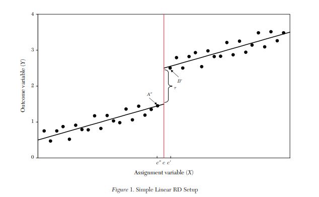
Regression Discontinuity Designs
(RDD) are used to identify the impact
of interventions assigned to people on
the basis of an assessment of need or
appropriateness.
Comparison Group Treatment Group
Pictured is a line graph. The x-axis of the graph represents the range of scores on a pretest you
will use to determine who gets the intervention and who does not. The centered red vertical
line is the score cutoff separating the two groups – those scoring above the cutoff get the
intervention, those scoring below the cutoff do not and are the comparison group. The y-axis
represents the outcome of interest for the study. The relationship between scores and
outcomes is plotted and summarized by a regression line for each of the two groups. The kink
in the graph between the two groups is the treatment effect. That is, the relationship between
x and y is, on average, greater for those who got the intervention.
10Regression Discontinuity Designs
Regression Discontinuity Designs
(RDD) are used to identify the impact
of interventions assigned to people on
the basis of an assessment of need or
appropriateness.
Comparison Group Treatment Group
An RDD identifies the effect of an
intervention on an outcome by taking
advantage of the fact that the
intervention is assigned to a
person based on a cutoff score.
11Regression Discontinuity Designs
Regression Discontinuity Designs
(RDD) are used to identify the impact
of interventions assigned to people on
the basis of an assessment of need or
appropriateness.
Comparison Group Treatment Group
An RDD identifies the effect of an
intervention on an outcome by taking
advantage of the fact that the
intervention is assigned to a
person based on a cutoff score.
Comparing outcomes for the
people whose scores are on either side
of the cutoff shows the effect of the
intervention.
12WHAT’S NEW
Requirements for an RDD Evaluation
RDDs require that the process used to assign an individual to an intervention
meets the following criteria:
A continuous measure (i.e., test score, age) is used to identify the individuals to receive an
intervention. Examples in a child welfare setting could be a risk-assessment score or measure of
child behavior.
Example: A state agency uses foster parent assessments of children in their care using the Child Behavior
Checklist (CBCL) to assign children in foster homes to a wraparound services program intended to prevent group
care placement.
A clearly defined cutoff point, or threshold, above or below which an individual is determined to
be eligible for the intervention.
Example: Foster homes with children whose CBCL scores place them in the clinical range on the measure are
provided with the wraparound intervention, whereas children whose scores are not as high as the clinical cutoff
do not.
13WHAT’S NEW
Key Assumptions of RDD
The measure used to assign people to the intervention should be continuous around
the cutoff point.
For example, if those just above the cutoff score are seen as having a qualitatively
different need for help than those just below the cutoff, then RDD is not an
appropriate evaluation design.
The average characteristics of individuals close to the cutoff point should be very
similar to each other.
RDD assumes that the difference in outcomes between the treatment and comparison
groups near the cutoff point—in other words, the impact of the intervention—applies
equally to individuals whose score is far from the cutoff point
14WHAT’S NEW
Difference-in-Differences
Difference in differences (DID) takes
advantage of differences in the timing across
sites (e.g., states, counties, agency offices,
organizations) where interventions are
implemented to assess intervention impacts.
DID identifies the impact of an intervention on O
the people in sites where the intervention is U
implemented. It does this by comparing change T
C
over time in outcomes for the people in sites
O
that received the intervention to change over
M
time in outcomes for people in sites that did not E
receive the intervention.
Pictured is a line graph. The x-axis of the graph is time and the y-axis is the outcome. The vertical line is a point in time separating the period
before the intervention and the period after the intervention is implemented. The comparison group line in the pre period shows how the study
group performed on the outcome over time without the intervention. The treatment group line in the same pre period shows how that study
group performed over time with the intervention. The same lines are displayed during the “after”, or implementation period. If there is a
treatment effect, then there will be a kink in the line, i.e., a change in the average effect, for the treatment group occurring sometime after the
intervention started. The idea is that the comparison group may get better over time, but that the treatment group got “more better” over time.
That is, the rate of change was greater in the treatment group than the rate of change in the comparison group. TIME
15WHAT’S NEW
Under Ideal Conditions, DID Is Useful for Evaluating Site-Based
Interventions
DID requires the availability of outcome data measured from an intervention
group and a comparison group at two or more different time periods, at least once
before the intervention begins and at least once after treatment.
16WHAT’S NEW
Under Ideal Conditions, DID Is Useful for Evaluating Site-Based
Interventions
DID requires the availability of outcome data measured from an intervention group and a
comparison group at two or more different time periods, at least once before the
intervention begins and at least once after treatment.
Key assumptions of the design:
“Parallel Trends” in outcomes: Any differences in outcomes between the intervention and
comparison groups would have been the same over time in the absence of the intervention.
Having multiple measures of the key outcome(s) both before and after the time the
intervention began in both the intervention and control sites helps assess whether this
assumption is reasonable.
The choice of sites to receive the intervention should be unrelated to the outcome. For
example, don’t choose sites based on the perceived strengths or needs of the people there.
The characteristics of the populations in the intervention and comparison sites should remain
constant over time.
17WHAT’S NEW
Strengths of DID for Evaluating Policies and Programs
Strong case for a causal effect of an intervention when the assumptions
are met
Relatively easy to interpret impacts
Can be used to assess the impact of interventions at a “system” level
Groups can start at different levels of the outcome, since change in the
outcome is the focus
18WHAT’S NEW
Interrupted Time Series
In evaluation research, a time series is a sequence of measurements taken over
time of outcomes experienced by a group of people.
For example, a time series could be the number of children per thousand reported to child
protection authorities each month over a period of several years.
In an Interrupted Time Series (ITS) evaluation, the time series of an outcome of
interest is used to establish an underlying trend in that outcome, and the
evaluator assesses whether the level or slope of that trend is affected by the
implementation of an intervention.
19WHAT’S NEW
ITS Can Be a Strong Design for Evaluating Large-Scale Interventions
Pictured is a line graph. The x-axis of the graph is time and the y-axis is the outcome. A line on the left half of the graph
represents the slope of the relationship between an outcome and time. The line is horizontal so there is no
relationship, i.e., the outcome is constant over time. A line on the right half of the graph starts at a lower point on the
y-axis and slopes downward. The intervention was introduced at the time point in the middle. Together, these lines
show that the after the intervention was introduced, there was a decline in both the immediate outcome and an
ongoing decline over time.
20Your thoughts on the designs we have discussed so far…?
Matched Comparison Group Designs
What will you gain?
1. Learn what a matched group design is
2. Learn different approaches to matched group designs and key
considerations
3. Hear about a real-world example
4. Share with others the work you have done using a matched
comparison designMatched Comparison Group Designs
1. What is a matched comparison group design?
For every member of the treatment group, you match them with someone from the comparison
group.
You match them using characteristics of people—age, family size, and socioeconomic status, for
example.
2. Why do a matched comparison design? What problem does the method solve?
When studying the benefit of participating in an intervention or program, we have to ask
whether the treatment and comparison groups are different, especially if those differences are
related to the outcomes.
Matching a treatment group member to a comparison group member is a way to make the two
groups as similar as possible with the information you have about the people in the study.
A successful match means you can say with confidence that the intervention worked (or did not).
3. Matched comparison group designs can be used to determine whether an intervention or program
had an effect (or impact).
23Matched Comparison Group Designs—Option 1
Exact matching—as the name implies, each member of the treatment group is
matched to a comparison group member exactly on each variable used.
Treatment group member: female, age 30, married, income below poverty threshold,
depressed, etc.
Comparison group member: female, age 30, married, income below poverty threshold,
depressed, etc.
You can do an exact match by sorting the two populations in the same order.
24Matched Comparison Group Design—Option 2
Propensity score matching (PSM)—when exact matching is not possible, we
need a way to judge how similar the treatment and control groups are
With a PSM, you want to understand who goes into the treatment group and then
select comparison group members with the same “propensity.”
The propensity score measures the quality of the match.
The quality of the match is called “closeness” or how much alike are the treatment
and comparison groups.
You can use the same variables as with exact matching.
PSM is more technical—all the major statistical software platforms have PSM
tools: SAS, SPSS, STATA, R, etc.*
*Software for Implementing Matching Methods and Propensity Scores,” Elizabeth Stuart’s Propensity Score
25
Software Page, Accessed June 20, 2020, http://www.biostat.jhsph.edu/~estuart/propensityscoresoftware.html.Matched Comparison Group Designs—Which Approach
Should I Pick?
1. Choosing the approach—exact match or PSM
How many variables should you use for the match?
No precise definition, but more variables is better
However…too many variables makes exact matching difficult
The process is iterative—best to think of the options as both/and rather than either/or
The goal is the best possible match—your judgment is important, but also consult with an
expert
Start with an exact match
View the results to examine the quality of the match—this is about how close the matches are
How many treatment group members get dropped because there is no match is an
important question
Evaluate your options—settle on the exact match or move onto PSM
26Matched Comparison Group Designs—
What Matching Variables Should I Use?
1. A matching variable is a characteristic of a person. The matching variable is used to find
someone in the comparison group who looks like a member of the treatment group.
2. Choosing the matching variables:
Variables used in the match should be correlated with the outcomes.
Age (a matching variable) is negatively correlated with adoption (the outcome): older children
are less likely to be adopted. Age is a good matching variable because of that connection.
Outcomes variables should not be used for the match.
Do not match the treatment group member to a comparison group member based on whether
they were adopted.
Be liberal in the choices you make—when you ask yourself whether to include a variable in
the match, the answer is yes so long as it is not an outcome.
27Matched Comparison Designs—Other Considerations
1. Administrative data (e.g., SACWIS / CCWIS) is an important resource for QEDs
Large number of subjects—thousands if not many more
2. May need to integrate those basic admin data with other information about an
intervention
Dates of intervention services, length of service, program fidelity measured in
terms of attendance
Data from other public programs could be a good source of matching variables
(e.g., TANF receipt, Medicaid service histories)
3. Once the data file with the matched treatment and comparison group members
has been assembled, you will have to use matching variables in your statistical
models.
28Describe a Real-World Example of a Matched Comparison
Design in Child Welfare
1. Intercept™ is a placement prevention intervention implemented in Tennessee.
2. It’s evaluated with a QED based on exact matching:
age, gender, race/ethnicity, clinical profile, socioeconomic needs, factors related to the risk
of placement following a report;
matching results were very good—lost very few treatment group members.
3. Data came from linked administrative data:
child protective investigations, placement, assessment, and services enrollment;
also linked each child to the worker who managed the case; and
also considered the county where the child was living at the time of removal.
We found that Intercept had a positive impact on placement prevention—57 percent
reduction in placement.
29Questions and Answers
This report is in the public domain. Permission to reproduce is not necessary. Suggested citation: Urban
Institute et al. (2021). Slide Deck Session 8: Quasi-Experimental Evaluation Designs - Child Welfare
Evidence-Building Academy. OPRE Report 2021-114, Washington, DC: Office of Planning, Research and
Evaluation, Administration for Children and Families, U.S. Department of Health and Human Services.You can also read