Question Type Classification Methods Comparison
←
→
Page content transcription
If your browser does not render page correctly, please read the page content below
Question Type Classification Methods Comparison

                                                                             Tamirlan Seidakhmetov
                                                                               Stanford University
                                                                            tamirlan@stanford.edu
arXiv:2001.00571v1 [cs.CL] 3 Jan 2020

                                                                                     Abstract

                                                 The paper presents a comparative study of state-of-the-art approaches for question
                                                 classification task: Logistic Regression, Convolutional Neural Networks (CNN),
                                                 Long Short-Term Memory Network (LSTM) and Quasi-Recurrent Neural Net-
                                                 works (QRNN). All models use pre-trained GLoVe word embeddings and trained
                                                 on human-labeled data. The best accuracy is achieved using CNN model with five
                                                 convolutional layers and various kernel sizes stacked in parallel, followed by one
                                                 fully connected layer. The model reached 90.7% accuracy on TREC 10 test set.
                                                 All the model architectures in this paper were developed from scratch on PyTorch,
                                                 in few cases based on reliable open-source implementation.

                                        1 Introduction

                                        Text classification is a popular task in NLP which has a wide range of applications, such as doc-
                                        ument classification and question classification task. The latter task is an essential part of general
                                        question-answering and named entity recognition algorithms. With the recent progress of the artifi-
                                        cial intelligence, tremendous progress has been made in this field, as when a question is asked, it is
                                        crucial to understand what the question is about before proceeding to answer search.
                                        This paper focuses on short questions classification task and provides a comparative study on the
                                        state-of-the-art approaches in this field, such as QRNN, CNN, and LSTM models. All models are
                                        trained and tested on TREC 10 dataset.

                                        2 Related work

                                        Multiple attempts have been made to design various deep learning methods for text classification
                                        tasks and compare their performances on various questions. Le-Hong and Le in their work com-
                                        pared Convolutional Neural Networks (CNN), Recurrent Neural Networks (RNN), Long Short-Term
                                        Memory Network (LSTM) and Feed-Forward Neural Network (FNN) on two datasets: UIUC En-
                                        glish question classification dataset with fine-grained 50 classes and Vietnamese sentences from
                                        the vnExpress online newspaper [1]. While paper gives good insights on how performances of dif-
                                        ferent architectures compared, it did not consider novel Quasi-Recurrent Neural Network (QRNN)
                                        architecture.
                                        The original QRNN paper also tried to compare their model with different variations of RNN, LSTM
                                        and CNN architectures. They used the IMDB movie review dataset to see how QRNN performs
                                        against other state-of-the-art models. One of the reported advantages of QRNN is that it performs
                                        well on longer text, however, researchers did not publish any results on QRNN’s performance on
                                        shorter sentence classification [2].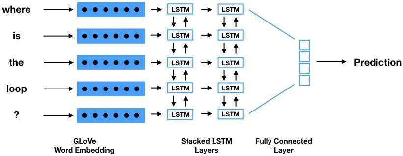
3 Approach
3.1 Data pre-processing
Firstly, all individual words and punctuation like question marks and commas in the question sen-
tence were tokenized into separate entities.
Xword = [token1, token2, ..., tokenN ] ∈ Z N
where N is a number of tokens in the sentence.
After that, the words have been converted to word indices and then further converted to word embed-
dings using GLoVe pre-trained word vectors. The GLoVe vectors were pre-trained using 840 billion
tokens from Common Crawl, and each token is mapped into a 300-dimensional vector [3].
Xembeddings = GloveEmbedding(Xword) ∈ RN xDword
where Dword is a number of dimensions of a word vector. Using these input features various models
have been built.
3.2 Logistic Regression
As a baseline, a multi-class logistic regression model has been built. After each word was converted
to Dword = 300 dimensional word vector, the input became N xDword , where N is a number of
words in a sentence. Then, the average pooling was applied per each sentence along each dimension,
so that the output became a 1xDword dimensional vector.
Xavg = AverageP ool(Xembeddings) ∈ RDword
Further, one layer of linear network has been applied followed by a Sigmoid function, which is
equivalent to logistic regression.
Xprob = Sigmoid(LinearLayer(Xavg)) ∈ RC
The output is a C-dimensional output, where C is a number of classes that we are trying to predict,
and the output value is a probability of each class. The code for the baseline model was implemented
from scratch.
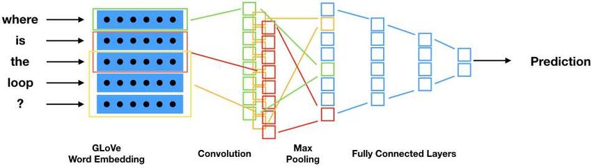
3.3 Convolutional Neural Network
Convolutional Neural Network (CNN) is a popular building block for many neural networks and
widely used in image processing. Here CNN was implemented on the question classification task
based on Yoon Kim’s “Convolutional Neural Networks for Sentence Classification” research work
[4]. After the words have been converted to word embeddings, a series of convolution layers have
been applied in parallel, with various kernel sizes K. Different kernel sizes correspond to various
n-grams, so when kernel size is 2, the model looks for 2-grams, therefore learning a lower term
meaning of words, whereas, for kernel size 5, CNN learns 5-grams which have higher term informa-
tion about the question. The number of kernels, as well as their sizes, are important hyperparameters,
that were tuned to find an optimal setting.
Xconv_k = Conv(Xembeddings), k ∈ K
Further, the outputs of all convolution layers with different kernel sizes are passed through the max-
pooling step over time.
Xmaxpool_k = M axP ool(Xconv_k), k ∈ K
Then the results are stacked together.
Xmaxpool_all = Stack(Xmaxpool_k), k ∈ K
During training time, the dropout layer is implemented for regularization. This step is omitted at
inference time.
Xmaxpool_all = Dropout(Xmaxpool_all)
2Finally, the output is passed through the fully connected layer and then a Softmax function. The
output vector represents the probability scores of each output class.
Xlinear = LinearLayer(Xmaxpool_all)
Xprob = Sof tmax(Xlinear)
Several experiments have been conducted to improve the original implementation of the CNN archi-
tecture in Yoon Kim’s paper, specifically multiple fully connected layers were added at the end, to
increase the complexity of the model and improve the accuracy. So the last two layers looked like
the following:
Xlinear1 = LinearLayer(Xmaxpool_all)
Xlinear2 = LinearLayer(Xlinear1)
Xlinear3 = LinearLayer(Xlinear2)
Xprob = Sof tmax(Xlinear3)
Each subsequent linear layer decreased the output size by half, except for the last one, which still
has an output size equal to the number of classes that the model needs to predict.
The code for this part was inspired by similar open-source implementation of the CNN model [5],
along with modifications in neural network architecture and hyperparameter tuning.
Figure 1: CNN Architecture with 3 FC layers
3.4 Long Short-Term Memory Network
Long Short-Term Memory (LSTM) Network is a popular type of Recurrent Neural Networks (RNN),
which became an essential building block for many neural network architectures. LSTM layers are
frequently used in a bidirectional setup with multiple layers stacked together, to learn higher-level
dependency of the words in a sentence. A similar work was done by Yangyang Shi and others, where
they fed word embeddings into multiple stacked bi-LSTM layers and used the convolution layer
across different bi-LSTM layers to capture features at different layers. Then the model followed by
average pooling [6].
In our work, the convolutional layer is not used, as to test the capabilities of LSTM only model. The
word embeddings are fed to multiple stacked bidirectional LSTM networks with dropout applied in
between:
Xlstm1 = BiLST M1(Xembeddings)
Xlstm1 = Dropout(Xlstm1 )
Xlstm2 = BiLST M2(Xlstm1 )
Xlstm2 = Dropout(Xlstm2 )
...
Xlstmn = BiLST Mn(Xlstmn−1 )
Xlstmn = Dropout(Xlstmn )
3The product of stacked Bi-LSTM layers is passed through a fully connected linear layer, followed
by a softmax function to obtain the prediction probability of each class.
Xprob = Sof tmax(LinearLayer(Xlstmn))
The output is C-dimensional vector, where C is a number of classes
The code for this part is implemented from scratch.
Figure 2: LSTM Architecture with 2 stacked Bi-LSTM layers
3.5 Quasi-Recurrent Neural Network
Quasi-Recurrent Neural Networks is a relatively new approach for modeling a sequence data, intro-
duced by James Bradbury and others at Salesforce in 2017 [2]. QRNN is a novel model, which uses
the advantages of previously well known two models: LSTM and CNN. While LSTM is good at
capturing dependencies in sequential data for moderately long sequences, it frequently fails to per-
form well on very long sequences such as document and paragraph classification, or character-level
models. Also, it has relatively slow performance, due to inability to do parallel computations. On
the other hand, CNN allows faster computation, as convolution operations could be done in parallel,
those allowing better scaling. QRNN tries to capture long term dependencies and allows parallelism,
which is good for scaling [2].
QRNN consists of two sub-components: convolution and max-pooling, both of which are paralleliz-
able. At a time step t, a convolution filter with filter width k is applied, starting from xt−k+1 to xt ,
mainly to be used at the next element in a sequence prediction tasks. A total of m convolution filters
are applied as described above, followed by tanh nonlinearity. Forget and output gates with sigmoid
functions are used at the pooling step.
Overall, the neural network architecture of QRNN model in this paper is similar to LSTM architec-
ture in previous section, except bidirectional LSTM is replaced by unidirectional QRNN layer with
a convolution filter width 1 and 2:
Xqrnn1 = QRN N1 (Xembeddings)
Xqrnn1 = Dropout(Xqrnn1 )
Xqrnn2 = QRN N2 (Xqrnn1 )
Xqrnn2 = Dropout(Xqrnn2 )
Xprob = Sof tmax(LinearLayer(Xqrnn2 ))
The code in this part was implemented from scratch, except the QRNN module itself, which has an
official open-source implementation by the authors of the paper.
44 Experiments
4.1 Data
TREC question classification dataset was used to compare the methods. It provides questions that
mostly consist of one sentence and target is one of six classes associated with the question: Abbre-
viation, Entity, Description, Human, Location and Numeric. Here are the examples of questions in
each class:
Table 1: TREC dataset quesion-class examples
Question Class
Who killed Gandhi? Human
What does the abbreviation AIDS stand for? Abbreviation
What do Mormons believe? Description
What is the date of Boxing Day? Number
What is a female rabbit called? Entity
Where is the highest point in Japan? Location
There are a total of 5500 training examples and 500 test examples. The training set was further
separated into 4500 training, 500 validation and 500 preliminary test examples.
4.2 Evaluation method
The model is being evaluated using an accuracy score, which is defined as:
X true labels
Accuracy =
all predicted labels
True labels are correctly predicted values.
4.3 Experimental details
For data preparation, a torchtext text preprocessing library for PyTorch has been used. The library
helps with building a word vocabulary, separate data into training, validation and test sets, convert
tokenized sentences to indices, apply padding and build an iterator to iterate over batches. The
iterator also separates sentences into batches by their lengths, so that shorter sentences appear next
to shorter ones in the same batch, and minimal padding is applied. One deficiency of the library is
that there is no way to apply padding to a sentence and have a predefined minimum sentence length,
which is needed when CNN with larger kernel sizes is applied. For instance, when kernel size is
5, and maximum sentence length in a batch is 4, the model needs padding. Therefore padding and
tokenization logic was implemented from scratch.
After the input pre-processing, GLoVe 300-dimensional pre-trained word vectors have been loaded
to the Embedding layer. Also, Adam optimizer has been used at a training stage. The batch size is
64.
Both TREC and Books model training is done on GPU, due to training data sizes. All the models
have been trained for 30-100 epochs, depending on the training data size.
The dropout rates used in the experiment range between 0.2-0.7 and the hidden layer size between
50 and 300.
The training time of each model is around 20 min for the TREC dataset, and up to 10-15 hours for
Books dataset on GPU.
4.4 Results
Table 2 shows a comparison of performances of CNN architectures with various kernel size combi-
nations. It could be noted that as higher-level kernels are appended to the model, the accuracy gets
5better at the beginning and then plateaus: after reaching sizes 5 or 6, there is no much incremental
increase. One possible reason for this is that many question sentences in the dataset are relatively
short, and most of their meanings are captured by lower-level kernels. So two best CNN models
with four (2,3,4,5) and five (2,3,4,5,6) kernel sizes are chosen to be further tested.
Table 2: CNN kernel size comparison on TREC Internal Test Set
Model Accuracy
CNN w kernels (2) 85.8
CNN w kernels (2, 3) 87.2
CNN w kernels (2, 3, 4) 87.6
CNN w kernels (2, 3, 4, 5) 88.8
CNN w kernels (2, 3, 4, 5, 6) 88.8
Table 3 below shows the comparison among different algorithms on TREC 10 and Books app test
sets:
Table 3: Test set comparison
Model TREC 10 Accuracy
Logistic Regression 87.3
Bi-LSTM - 2 Stacked Layers 88.3
Bi-LSTM - 5 Stacked Layers 82.4
CNN w kernels (2,3,4,5) + 1 FC Layer 89.6
CNN w kernels (2,3,4,5,6) + 1 FC Layer 90.7
CNN w kernels (2,3,4,5,6) + 3 FC Layers 88.6
QRNN w 1 Layers and Window Size 1 77.8
QRNN w 2 Layers and Window Size 1 86.2
QRNN w 2 Layers and Window Size 2 88.0
Baseline Logistic Regression model shows very good performance on TREC 10 dataset, however,
2-layer stacked Bi-LSTM model performs a little better, improving a baseline result by 1%.
CNN based approach with kernel sizes from 2 to 6 and one fully connected layer shows the best
performance among all models, reaching 90.7% accuracy.
More complex QRNN model does well on TREC 10, but simpler alternatives do not perform well
on this dataset, trailing behind the baseline model. This might be due to a small training data size
for this task.
5 Analysis
The models’ comparison is shown in Table 3. Here are a few frequent errors that models do:
1. Classify text with names as "human".
2. Out-of-vocabulary words. There is a special embedding for all out-of-vocabulary words,
it means the model sees all out-of-vocabulary words similarly. This decreases the perfor-
mance of the models. The problem mostly affects unusual names and new or foreign words.
3. Misspelling. This is a subset of an out-of-vocabulary word problem, however, this problem
worth a separate bullet point, as people tend to misspell frequently.
6References
[1] Phuong Le-Hong and Anh-Cuong Le. A comparative study of neural net-
work models for sentence classification. CoRR, abs/1810.01656, 2018. URL
http://arxiv.org/abs/1810.01656.
[2] James Bradbury, Stephen Merity, Caiming Xiong, and Richard Socher. Quasi-recurrent neural
networks. CoRR, abs/1611.01576, 2016. URL http://arxiv.org/abs/1611.01576.
[3] Jeffrey Pennington, Richard Socher, and Christopher D. Manning. Glove: Global vectors for
word representation. In Empirical Methods in Natural Language Processing (EMNLP), pages
1532–1543, 2014. URL http://www.aclweb.org/anthology/D14-1162.
[4] Yoon Kim. Convolutional neural networks for sentence classification. CoRR, abs/1408.5882,
2014. URL http://arxiv.org/abs/1408.5882.
[5] threelittlemonkeys. Cnns for text classification in pytorch.
https://github.com/threelittlemonkeys/cnn-text-classification-pytorch,
2019.
[6] Yangyang Shi, Kaisheng Yao, Le Tian, and Daxin Jiang. Deep lstm based feature mapping for
query classification. pages 1501–1511, 01 2016. doi: 10.18653/v1/N16-1176.
7You can also read