Deep Graph Convolutional Networks for Wind Speed Prediction
←
→
Page content transcription
If your browser does not render page correctly, please read the page content below
ESANN 2021 proceedings, European Symposium on Artificial Neural Networks, Computational Intelligence
and Machine Learning. Online event, 6-8 October 2021, i6doc.com publ., ISBN 978287587082-7.
Available from http://www.i6doc.com/en/.

          Deep Graph Convolutional Networks for Wind
                      Speed Prediction
                            Tomasz Stańczyk and Siamak Mehrkanoon

          Maastricht University - Department of Data Science and Knowledge Engineering
                  Paul-Henri Spaaklaan 1, 6229 EN Maastricht - The Netherlands

             Abstract.      In this paper, we introduce a new model for wind speed
             prediction based on spatio-temporal graph convolutional networks. Here,
             weather stations are treated as nodes of a graph with a learnable adjacency
             matrix, which determines the strength of relations between the stations
             based on the historical weather data. The self-loop connection is added
             to the learnt adjacency matrix and its strength is controlled by additional
             learnable parameter. Experiments performed on real datasets collected
             from weather stations located in Denmark and the Netherlands show that
             our proposed model outperforms previously developed baseline models on
             the referenced datasets.

      1     Introduction and Related Work
      Deep learning based models have been successfully applied for weather elements
      forecasting [1–3]. Although Long Short-Term Memory (LSTM) recurrent net-
      works [4], work well for time series prediction [5], they do not explicitly include
      spatial relations within the data. Authors in [6] combined LSTM with convo-
      lutions to create ConvLSTM, which was used for precipitation tasks, while also
      capturing the data spatial structure. The authors in [3] introduced convolutional
      neural network (CNN) models based on 1D-CNNs for multi-source 1D weather
      data, 2D- and 3D-CNNs to process the tensor-form 3D weather data. In this
      way, the spatial-temporal relations were extracted with 2D and 3D CNNs. The
      authors in [7] proposed using depthwise-separable convolutions to process differ-
      ent dimensions of the input tensor and then concatenating resulting tensor along
      single dimension. However, all the CNN-based models above discard the spatial
      relations between the cities (weather stations). In other words, these approaches
      process input tensor, where neighborhood of the cities is determined only by the
      order of the cities in the tensor or the dataset.
          Graph convolution networks (GCNs), which are a particular type of graph
      neural networks [8] can generalize CNNs to work on graphs rather than on
      regular grids [9]. In particular, it enables incorporating the neighbor relation
      information, e.g. through an adjacency matrix of a graph. The authors in [10]
      introduced weighted graph convolutional LSTM architecture, which combines
      LSTM with matrix multiplications replaced with graph convolutions with a sin-
      gle (one for the whole model), learnable adjacency matrix. In [11], the authors
      created a graph based on the wind farms and for each node of the graph, tem-
      poral features were extracted with LSTMs.

                                                 147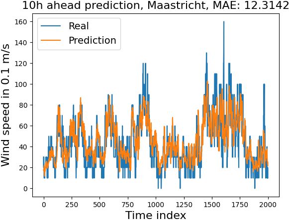
ESANN 2021 proceedings, European Symposium on Artificial Neural Networks, Computational Intelligence
and Machine Learning. Online event, 6-8 October 2021, i6doc.com publ., ISBN 978287587082-7.
Available from http://www.i6doc.com/en/.

          In this work, we treat weather stations and their corresponding weather
      variable values from different time steps as a spatio-temporal graph, as pre-
      sented in Fig. 1(c). Here, we develop our own novel model from ST-GCN [12]
      and 2s-AGCN [13] architectures which were successful on skeleton-based action
      recognition tasks. In particular, we include learnable parameter controlling the
      self-connection strength of the learnt adjacency matrix and normalize the matrix.
          This paper is organized as follows. Section 2 presents the proposed model
      and relevant details. Section 3 describes the conducted experiments with corre-
      sponding results. Finally, conclusions are drawn in Section 4.

      2     Methods
      In this work we experiment on two Dutch and Danish datasets. The data con-
      sists of historical observations (time steps) for several cities and several weather
      variables. The aim is to predict the wind speed values for selected cities for
      several time steps ahead. At a single time step, we treat the input cities as a
      graph where each city is a node in the graph. Node attributes are then weather
      variables for the first layer of the network and features encoded by the network
      in the next layers. For the cities shown in Fig. 1(a), at a single time step, the
      corresponding spatial graph could be perceived as in Fig. 1(b).

                          (a)                   (b)                     (c)
      Fig. 1: (a) Map with the Danish weather stations. Possible: (b) spatial graph;
      (c) spatial-temporal graph; built from Danish weather stations.
          In practice, time series of historical data involve multiple time steps. There-
      fore, we include this information by expanding the previous graph into a spatial-
      temporal graph as shown in Fig. 1(c). Two types of convolutions are included in
      our proposed models, i.e. graph spatial convolution and temporal convolution.

      2.1    Graph Spatial Convolution
      Spatial convolution aggregates the information from the spatial neighbors of the
      graph. The graph is represented by an adjacency matrix. Following the lines
      of [10,13], we make the adjacency matrix learnable. During the optimization, the
      network learns the graph spatial connections between the weather stations. It
      should be noted that since all the entries are learnt in an end-to-end fashion, the
      adjacency matrix is not symmetric. The learnable adjacency matrix is further

                                                 148
ESANN 2021 proceedings, European Symposium on Artificial Neural Networks, Computational Intelligence
and Machine Learning. Online event, 6-8 October 2021, i6doc.com publ., ISBN 978287587082-7.
Available from http://www.i6doc.com/en/.
transformed during the training. Operations similar to those from GCNs of
[14], involving adding the self-loop connection and normalization with degree
matrix are applied. To the best of our knowledge, it is the first time to apply
such transformations over the adjacency matrix which is learnable. The new,
transformed matrix is created as follows. Self-loop connection in the form of
an identity matrix is added to the learnable adjacency matrix: Â = A + γI.
Here, γ is a learnable scalar parameter which lets the network decide about
the strength of the imposed self-loop connection. The resulting matrix  is
then scaled as follows: Â = Â Â−Âmin
. A diagonal node degree matrix D̂ is
max −Âmin
P
computed based on the normalized matrix: D̂ii = j Âij . Next, we apply the
1 1
symmetric normalization [14]: D̂− 2 ÂD̂− 2 . The resulting transformed matrix is
used for the graph convolution operation. Input data tensor Xin with the shape
of C × T × V , where C = #channels (weather variables), T = #timesteps
and V = #graph vertices (cities) is reshaped into a matrix Xin with dimension
of CT × V . The graph convolution is initially performed by multiplying the
reshaped input matrix with the transformed adjacency matrix:
1 1
Xout = Xin (D̂− 2 ÂD̂− 2 ). (1)
Next, the output matrix Xout is reshaped back into a tensor Xout with the shape
of C × T × V . Finally, 1 × 1 convolution is performed in order to combine the
features channel-wise and to increase the number of channels.
2.2 Temporal Convolution
Temporal convolution aggregates the information from the temporal neighbors
in the graph. For each separate node and its features, information from the next
and/or previous time step is included. The temporal convolution is implemented
as a regular 2D convolution with filter of size k × 1. The value of k is set to
3, as this value was experimentally found to be optimal value for our models
regarding their performance on the validation sets of the used datasets.
(a) (b)
Fig. 2: (a) Spatio-temporal block (ST-block) used in our models. Figure inspired
by [13]. (b) Overview of the proposed model(s). The numbers above the blocks
indicate the number of input and output channels respectively.
Using spatial convolution and temporal convolution operations, we create
a spatio-temporal block (ST-block). As presented in Fig. 2(a), both spatial
149ESANN 2021 proceedings, European Symposium on Artificial Neural Networks, Computational Intelligence
and Machine Learning. Online event, 6-8 October 2021, i6doc.com publ., ISBN 978287587082-7.
Available from http://www.i6doc.com/en/.
and temporal convolution are followed by a batch normalization (BN) layer and
a ReLU activation function. In addition, a residual connection is added over
the whole block. Each block contains its own, separate, learnable adjacency
matrix. We stack three spatio-temporal blocks with the following number of
output channels: 16, 32 and 64. The last block is followed by 1 × 1 convolution
which reduces the number of channels to 4 before flattening. A fully connected
(FC) layer is added at the end of the network to obtain wind speed predictions
for target cities. The model architecture is presented in Fig. 2(b). We call
our proposed model WeatherGCNet. The following setup is applied in the
training phase. Batch size is set to 64. Adam optimizer is used with the default
value of learning rate set to 0.001. The number of input timesteps T processed
by our models is tuned on validation sets and set to 30.
3 Experimental Results
We consider two datasets for the task of wind speed prediction. The data comes
from weather stations located in Denmark and the Netherlands. The datasets
contain hourly measurements of several weather variables for several Danish and
Dutch cities. In this study, the prediction targets are set to wind speed of Esb-
jerg, Odense, Roskilde for the Danish dataset and Schiphol, De Bilt, Leeuwarden,
Eelde, Rotterdam, Eindhoven, Maastricht for the Netherlands dataset.
As a preprocessing step, both datasets are normalized using the min-max
normalization based on values coming from the corresponding training sets. The
discussed datasets have been previously introduced in [3] and [7]. We train
our model with two variants: with γ set to 1 and with γ learnt with other
parameters. We evaluate our model together with the other models presented
in [7]. The referenced models are trained and evaluated on the same datasets
using the same data splits as used for our model. We report mean absolute
error (MAE) for each model on the test set. The reported MAEs are obtained
by takingPthe average over all output cities. The MAE is defined as follows:
n
|y −yˆ |
M AE = i=1 n i i Here, n denotes the number of samples in the test set. yi
and yˆi denote ground truth and predicted value respectively.
We train the models for predicting wind speed over 6, 12, 18 and 24 hours
ahead for the Danish dataset and 2, 4, 6, 8 and 10 hours ahead for the Dutch
dataset. The obtained MAE scores on the test set are tabulated in Table 1. The
best scores are underlined for each prediction time for both datasets. For the
Danish dataset, the scores of the baseline models are taken from the original
paper [7]. For the Dutch dataset, the relevant scores of the baseline models are
initially unavailable. We use the authors’ publicly available code implementation
to perform appropriate training and collect the corresponding MAE scores.
It can be observed that the proposed model WeatherGCNet with its both
variants, when γ is set to 1 and when γ is learnt, outperforms all the other
baseline models. This is due to the fact that our model learns and incorporates
the spatial neighbor relations between the weather stations based on a graph
rather than a tensorial form used in [3, 7], where neighborhood is determined
150ESANN 2021 proceedings, European Symposium on Artificial Neural Networks, Computational Intelligence
and Machine Learning. Online event, 6-8 October 2021, i6doc.com publ., ISBN 978287587082-7.
Available from http://www.i6doc.com/en/.
Table 1: The average MAEs of evaluated models for wind speed prediction over
the Danish and Dutch cities datasets.
Model Denmark Netherlands
6h 12h 18h 24h 2h 4h 6h 8h 10h
2D 1.304 1.746 1.930 2.004 8.18 10.08 12.03 13.15 14.51
2D + Attention 1.313 1.715 1.905 1.950 8.10 10.09 11.83 13.10 14.13
2D + Upscaling 1.307 1.723 1.858 1.985 8.24 10.22 11.83 13.74 14.80
3D 1.311 1.677 1.908 1.957 8.05 10.15 11.93 13.01 14.24
Multidimensional 1.302 1.706 1.873 1.925 8.10 10.03 11.46 12.79 13.81
WeatherGCNet (γ=1) 1.279 1.638 1.777 1.869 7.96 9.97 11.16 12.30 13.33
WeatherGCNet (learnt γ) 1.267 1.616 1.767 1.853 7.97 9.74 10.99 12.44 13.55
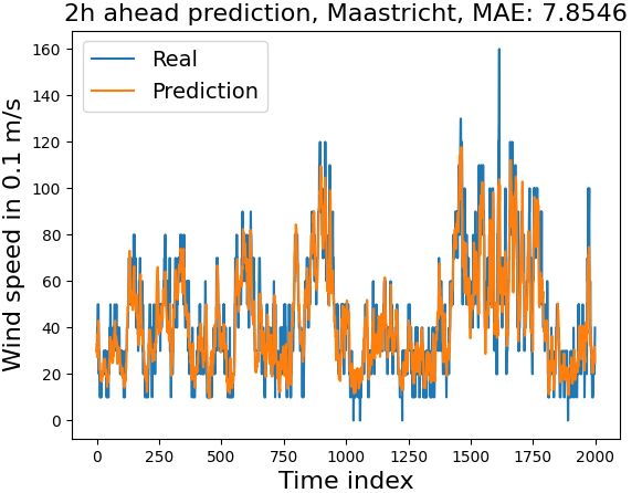
(a) (b)
Fig. 3: WeatherGCNet (γ=1) wind speed prediction plots for Maastricht (NL)
for: (a) 2h ahead, (b) 10h ahead.
only by the order of the cities in the dataset. Fig 3(a) and 3(b) show plots of
wind speed prediction obtained by the proposed model for the selected Dutch
city Maastricht. It should be noted that a subset of test data is used for plotting
whereas MAE scores included in the figures are reported for the whole test set.
Further, we also visualize the learnt adjacency matrices of the proposed model
for 2h ahead wind speed prediction for the Dutch dataset. Fig. 4(a) shows
the visualization of the adjacency matrix in the first spatio-temporal layer of
the WeatherGCNet model, where γ is set to 1. Fig. 4(b) shows analogous
visualization for model where the γ parameter is learnt. Given the possibility to
decide via the additional parameter, the network prefers the self-loop connection
to be relatively small (compared to the other entries), as visible in Fig. 4(b).
(a) (b)
Fig. 4: Adjacency matrix (first layer) visualization for wind speed 2h ahead
prediction on Dutch dataset. (a): Model with γ=1; (b): model with learnt γ.
151ESANN 2021 proceedings, European Symposium on Artificial Neural Networks, Computational Intelligence
and Machine Learning. Online event, 6-8 October 2021, i6doc.com publ., ISBN 978287587082-7.
Available from http://www.i6doc.com/en/.
4 Conclusion
In this paper, new model based on GCN architecture is proposed for wind
speed prediction using historical weather data. Thanks to the applied spatial-
temporal convolutional operations on the built graph, the network learns the
underlying relations between weather stations through a learnable adjacency
matrix of the graph. The self-loop connection of the adjacency matrix is en-
forced with and without learnable scalar parameter enabling the network to
decide about the strength of the self connectivity in the graph. Comparing
with previously introduced baselines, our proposed model provides more accu-
rate predictions in all cases examined. The github implementation is available
at https://github.com/tstanczyk95/WeatherGCNet.
References
[1] Sebastian Scher. Toward data-driven weather and climate forecasting: Approximating a
simple general circulation model with deep learning. Geophysical Research Letters, 45,
11 2018.
[2] Jesús Garcı́a Fernández, Ismail Alaoui Abdellaoui, and Siamak Mehrkanoon. Deep coastal
sea elements forecasting using u-net based models. arXiv preprint arXiv:2011.03303,
2020.
[3] Siamak Mehrkanoon. Deep shared representation learning for weather elements forecast-
ing. Knowledge-Based Systems, 179:120–128, 2019.
[4] Sepp Hochreiter and Jürgen Schmidhuber. Long short-term memory. Neural Computa-
tion, 9(8):1735–1780, 1997.
[5] Sima Siami Namini, Neda Tavakoli, and Akbar Siami Namin. A comparison of arima and
lstm in forecasting time series. ICMLA, pages 1394–1401, 12 2018.
[6] Xingjian Shi, Zhourong Chen, Hao Wang, Dit-Yan Yeung, Wai-kin Wong, and Wang-
chun Woo. Convolutional lstm network: A machine learning approach for precipitation
nowcasting. NIPS, pages 802–810, 2015.
[7] Kevin Trebing and Siamak Mehrkanoon. Wind speed prediction using multidimensional
convolutional neural networks. arXiv preprint arXiv:2007.12567, 2020.
[8] Franco Scarselli, Marco Gori, Ah Chung Tsoi, Markus Hagenbuchner, and Gabriele Mon-
fardini. The graph neural network model. IEEE Transactions on Neural Networks,
20(1):61–80, 2009.
[9] Si Zhang, Hanghang Tong, Jiejun Xu, and Ross Maciejewski. Graph convolutional net-
works: a comprehensive review. Computational Social Networks, 2019.
[10] T. Wilson, P. Tan, and L. Luo. A low rank weighted graph convolutional approach to
weather prediction. In 2018 IEEE International Conference on Data Mining (ICDM),
pages 627–636, 2018.
[11] M. Khodayar and J. Wang. Spatio-temporal graph deep neural network for short-term
wind speed forecasting. IEEE Transactions on Sustainable Energy, 10(2):670–681, 2019.
[12] Sijie Yan, Yuanjun Xiong, and Dahua Lin. Spatial temporal graph convolutional networks
for skeleton-based action recognition. AAAI, 2018.
[13] Lei Shi, Yifan Zhang, Jian Cheng, and Hanqing Lu. Adaptive spectral graph convolutional
networks for skeleton-based action recognition. CVPR, 2019.
[14] Thomas N. Kipf and Max Welling. Semi-supervised classification with graph convolutional
networks. ICLR, abs/1609.02907, 2017.
152You can also read