Future sea level projections - Tamsin Edwards Open University - eo science for society
←
→
Page content transcription
If your browser does not render page correctly, please read the page content below
Future sea level projections

      Tamsin Edwards
      Open University

                               1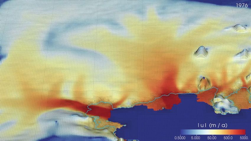
2
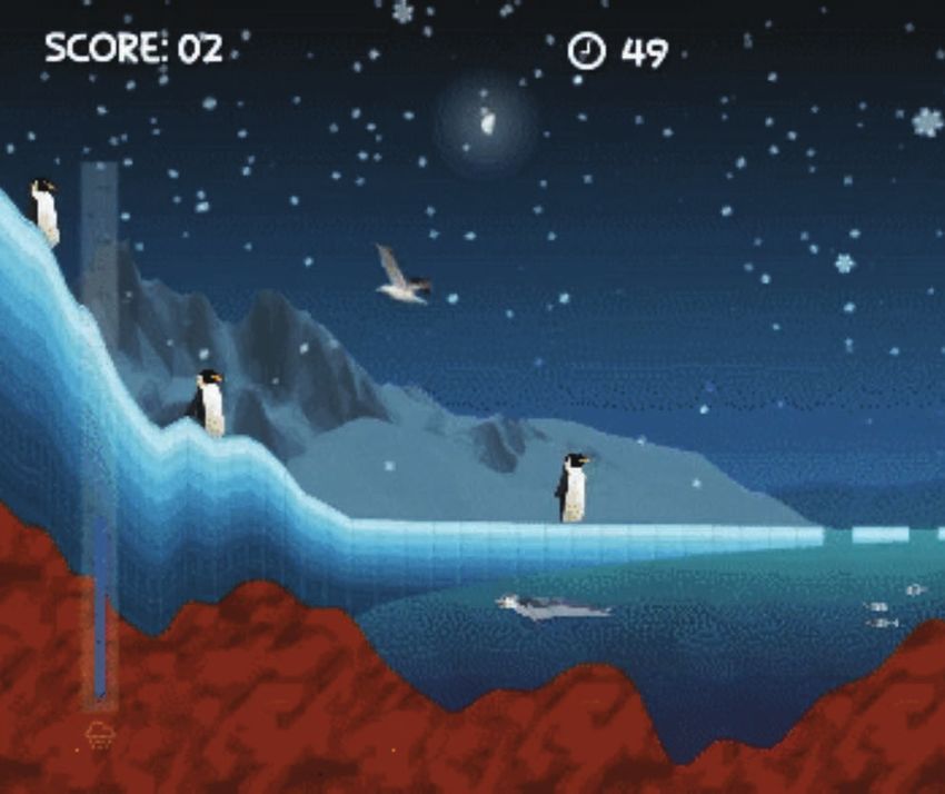
iceflowsgame.com 3 Developed by Anne Le Brocq
IPCC projections

      Global sea level rise                     74 [52, 98] cm
     relative to 1986-2005
                                                44 [28, 61] cm

                                             • Substantial sea level rise
                                               no matter what
               RCP8.5
                                             • Large uncertainties
             (exponential
              growth of
              emissions)

                RCP2.6 (strong mitigation)

Adapted from IPCC (2013) Working Group I Summary for Policymakers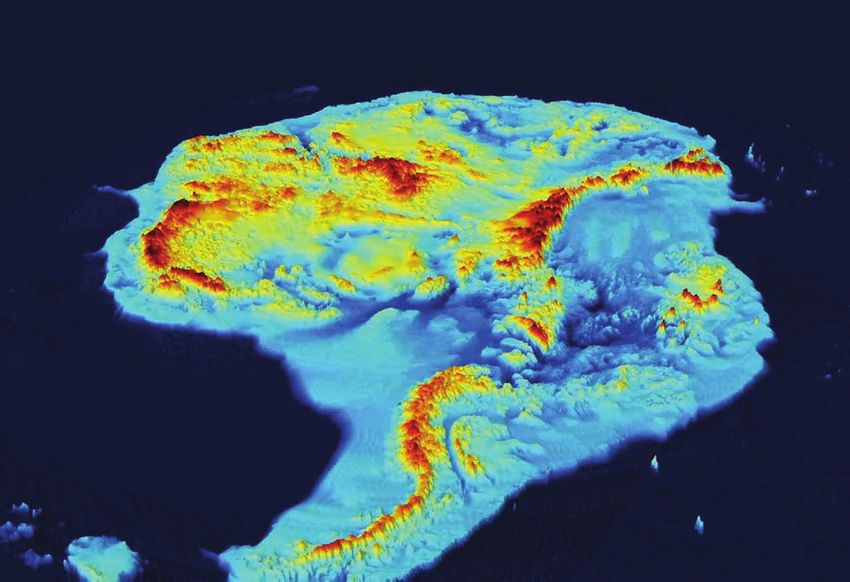
IPCC projections

      Global sea level rise                     74 [52, 98] cm
     relative to 1986-2005
                                                44 [28, 61] cm

                                             • Substantial sea level rise
                                               no matter what
               RCP8.5
                                             • Large uncertainties
             (exponential
              growth of
              emissions)                     • Ice sheets 1/4 or more

                                             • Antarctica the largest
                                               uncertainty: 7 [-1,16 cm]

                RCP2.6 (strong mitigation)   • Very poorly-constrained
                                               upper tail: 50 to 100 cm

Adapted from IPCC (2013) Working Group I Summary for Policymakers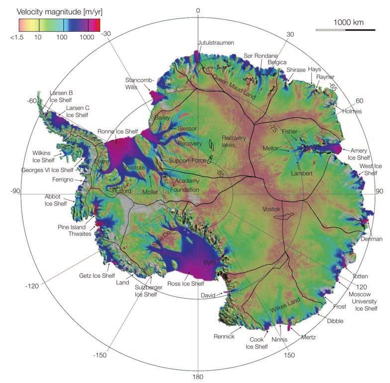
Ice sheet models
 •   flow of ice under its own weight                   Full Stokes
 •   different approximations
     of stress components

AntarcticGlaciers.org

                                         Shallow Ice
                                        Approximation

                                                                      6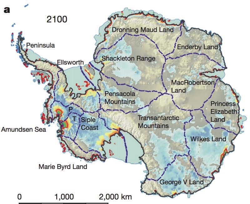
Ice sheet models
•   can calculate surface mass balance from atmosphere
    -   degree day models
    -   energy balance models
•   and/or basal mass balance from ocean               Source: Alexei Sharov
    -   melt parameterisation
                     Global climate model summer temp. anomalies
                     for 2091-2100 relative to 1989-2008
                     under SRES scenario A1B
                     (Goelzer et al., 2013)

                        Ocean model near-bottom
                        temperatures in 2150
                        under SRES scenario A1B
                        (Timmerman & Hellmer, 2013)
                                                                          7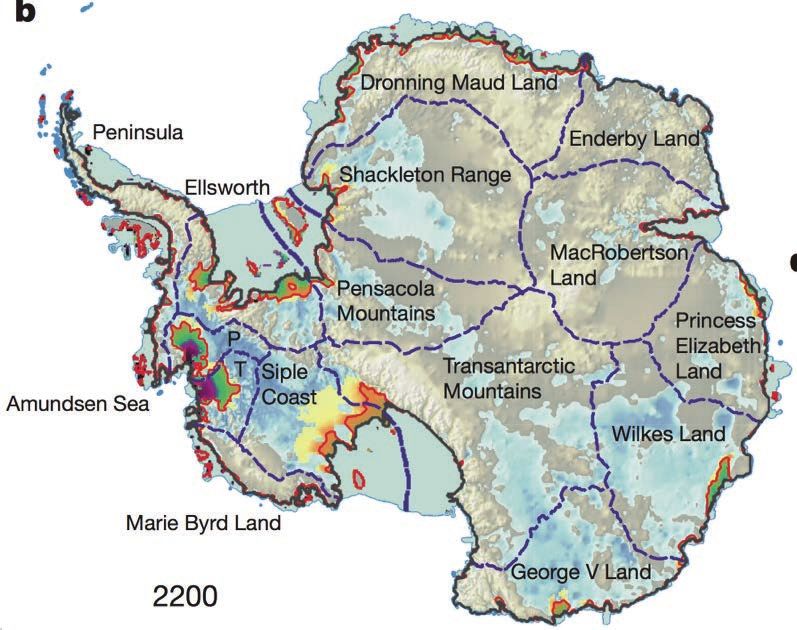
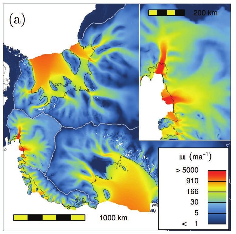
BISICLES

initial ice flow speed
(Cornford et al.,
2015)                    8
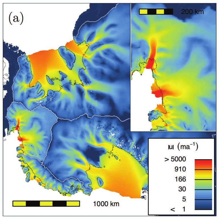
BISICLES

ice flow speed forced by ocean under SRES scenario A1B
(Cornford et al., 2015)                9
BISICLES

% mismatch between initial ice speed
and observations (Lee et al., 2015)    10
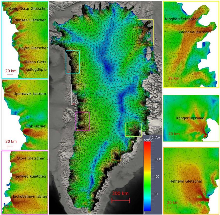
Elmer/Ice

initial surface velocities
(Gillet-Chaulet et al., 2012)    11
Elmer/Ice

initial surface velocities (Favier et al., 2014)          12
What is an ice sheet model used for?
 •   Understanding palaeoclimates

                                    Pliocene (3Ma BP)

Antarctic ice volume and
sea level equivalent
(Pollard and DeConto, 2009)

Pliocene ice sheet simulation
DeConto and Pollard (2016)                         13
What is an ice sheet model used for?
• Predicting the long-term future
“Antarctica has the
potential to contribute
…more than 15 m
[of sea-level rise] by
2500, if emissions
continue unabated.
…prolonged ocean
warming will delay its
recovery for thousands
of years.”
RCP8.5 ice sheet prediction at 2500
DeConto and Pollard (2016) 14What is an ice sheet model used for?
• Predicting the
short(ish)-term future
“Given sufficient melt rates,
we compute grounding line
retreat over hundreds of
kilometers in every major ice
stream, but the ocean
models do not predict such
melt rates outside of the
Amundsen Sea Embayment
until after 2100.”
grounding line migration in
ocean-forced simulations
(Cornford et al., 2015) 15Ice sheet predictions for policymakers
• Ice Sheet Model Intercomparison Project for CMIP6
- CMIP = Coupled Model Intercomparison Project Phase 6
• IPCC Sixth Assessment Report
- Published from 2020
• Range of complexities and computational expense
- Physics: full Stokes, various approximations
- Spatial resolution and domain
• Standalone and coupled with climate models
ISMIP6 design: Nowicki et al. (2016) 16How to use observations with models?
• Combining and comparing observations with models
- Both are imperfect
- Different spatial resolution, domains, variables
• To obtain best possible estimates of:
- system state: past, present and future ice sheet
- model parameters
All models!
are WRONG!
...but some are
USEFUL!
17How to use observations with models?
• Formal methods often derived from Bayes Theorem
1. model simulation(s) of state
2. compare with observations
3. update estimate of state and/or parameters
• e.g.
- Data Assimilation (state) - incorporating obs into simulations
- Bayesian calibration (parameters) - estimating parameters from
obs with Bayesian inference
• Less formal methods also used…
- ‘nudging’
- ‘relaxation’
- hand tuning
18What does an ice sheet model need?
1. Initial state
- ice sheet geometry
- ice velocity
- internal ice temperature
- basal traction coefficient
- maybe others, e.g.:
" enhancement factor
" effective viscosity, stiffness
" bedrock topography corrections
initial ice flow speed again
due to obs uncertainties (Cornford et al., 2015)
" mass balance corrections
to prevent artefacts/drift
19integrated effective viscosity
(Lee et al., 2015)
average effective viscosity
(Cornford et al., 2015)
20basal traction coefficient
(Lee et al., 2015; Cornford et al., 2015)
21synthetic mass balance
(Cornford et al., 2015)
22What does an ice sheet model need?
2. Boundary conditions
- bedrock topography, geothermal heat flux
bedrock elevation
(Bamber et al., 2013;
Morlighem et al., 2014) 23bedrock elevation: BEDMAP2
(Fretwell et al., 2013)
24geothermal heat flux (Shapiro et al., 2004; Rogozhina et al., 2012) 25
What does an ice sheet model need?
 3. Climate forcing or mass balance           -   observations
                                              -   climate models
    -   atmosphere:                           -   ice cores
        "   temperature & precipitation, or
                                              -   schematic

        "   surface mass balance (SMB)
                                              Basal melt rates in 2140-2149
    -   ocean                                 under SRES scenario A1B
        "   temperature, or                   (Timmerman & Hellmer, 2013)

        "   basal melting

Regional climate model SMB
anomalies for 2091-2100
relative to 1989-2008
under SRES scenario A1B
(Goelzer et al., 2013)                                                   26
Earth Observations
recent past now
!"#$% &$!$% future
&!""%
Initialisation
'()*+,)-+*.(% Evaluation
/+,)0+*.(%% Prediction
1230)4*.(%%
need Earth Observations here
27Initialising an ice sheet model
• Need to find self-consistent values for ice sheet state
- geometry, flow, ice temperature, basal traction coefficient, …
• Consistent with observations and reconstructions
- EO: geometry, elevation changes, velocities
- recent climate, reconstructed palaeoclimate
• Even though both are imperfect
• Data assimilation of various kinds, e.g.:
- tuning and inverse methods to estimate basal traction coefficient
from surface or balance velocities
- setting geometry equal to observed, then allowing model to ‘relax’ to
quasi-equilibrium state
28BEDMAP2 ice thickness (Fretwell et al., 2013) 29
surface elevation
(Howat et al., 2014)   30
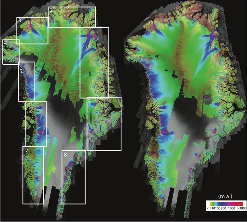
ice velocity
(Rignot et al., 2011)   31
ice velocity
(Joughin et al., 2010)   32
Estimating basal traction coefficient
 minimise mismatch
 between modelled and
 observed velocities

 e.g. cost function

observed and initial model
surface velocities
(Gillet-Chaulet et al., 2012)             33
Estimating basal traction coefficient
  inversion gives estimate of basal traction coefficient

initial average velocities               initial log(effective basal traction coeff.)
(Ritz et al., 2015)                                                                     34
Large initialisation uncertainties
•   Different methods
    -   formal vs ad-hoc
    -   free vs fixed geometry spin-up
    -   glacial-interglacial cycle(s) vs recent climatology
    -   mass balance corrections vs subtracting drift from predictions
•   Different datasets and time periods
    -   sometimes multiple variants
    -   mismatches in time coverage
    -   definition of “recent” climatology
•   Different model structures
    -   derive different initial states even if same method and data
                                                                         35
initialisation methods in ice2sea project Edwards et al., 2014) 36
How much does it matter?
•   Short-term ice sheet prediction like weather not climate
    -   ice sheet responds on centennial timescales
    -   decadal-century scale response depends strongly on initial state
•   Drift if no mass balance corrections
    -   subtract from predictions
•   More important than ever
    -   robust decadal-century scale
        predictions for adaptation

                      Greenland model drift
                      (Goelzer et al., 2016, EGU abstract)                 37
How much does it matter?
• Initial accumulation from:
- regional climate model
- initialisation: mass balance
corrections inferred for this climate
“Within the Amundsen Sea Embayment
the largest single source of variability is the
onset of sustained retreat in Thwaites
Glacier, which can triple the rate of
eustatic sea level rise….depends strongly
on its initial state”
Cornford et al. (2015) 38How much does it matter?
• Greenland ice sheet
- 500 years of A1B scenario
• glacial-interglacial cycle spin-up
- fix geometry to observed or allow to evolve freely?
fixed grey =
SeaRISE
ensemble
range
free
Saito et al. (2016) 39initMIP
• “Requirements”
- Participants can and are encouraged to contribute with different…
initialisation methods
- The choice of model input data is unconstrained to allow
participants the use of their preferred model setup without
modification.
- The specific year of initialization (between 1950 and 2014) is equally
unconstrained
See ISMIP6 wiki for more details 40initial ice thickness (Goelzer et al., 2016, EGU abstract) 41
evaluating an ice sheet model

                                42
Evaluating an ice sheet model
• Important!
- tests model adequacy
- can quantify model uncertainty
• Not much formal statistical inference out there
- only arbitrary comparisons e.g. RMSE
• Calibrating models in statistical framework
- use ensemble of simulations with different input values and fields
- compare with observations
- update knowledge about good/bad parameter values
• Ad-hoc methods also used
43Model calibration statistical frameworks
• History matching
- rule out poor versions of model to give confidence intervals
• Bayesian calibration
- highest weights to best versions to give probability distributions
What if:
obs = dog
model = cats?
• Strengths and weaknesses
- HM: “this model can’t simulate dogs”
- BC: “here is the cat that looks most like a dog”
“…but here is my uncertainty about that answer”
44History matching: Pine Island Glacier
1. model ensemble 95% confidence set
5000 simulations
varying 7 parameters
2. observations
grounding line
thickness
velocity
grey = ruled out
3. choose metric
(implausible)
4. define threshold
Gladstone et al. (2012) 45Bayesian calibration: Antarctica
1. model ensemble SLE
at 2200
3000 simulations (cm)
varying 16 inputs
2. observations
Amundsen Sea Embayment
mass trend (IMBIE)
3. choose likelihood
4. normalise and reweight
Ritz et al. (2015) 46Amundsen Sea Embayment mass trend (1992-2011)
Expected trend:
inc model error
Shepherd et al. (2012) 47Amundsen Sea Embayment at 2100 vs recent mass trend Ritz et al. (2015) 48
Amundsen Sea Embayment at 2200 vs recent mass trend

Ritz et al. (2015)                                      49
Weights ensemble members

       darkest =
    highest weight
  (highest likelihood)

Ritz et al. (2015)           50
Effect of calibration on sea level projections
2100 2200
calibrated
calibrated
uncalibrated
uncalibrated
Ritz et al. (2015) 51Probability of grounding line retreat at 2100 Ritz et al. (2015) 52
Probability of grounding line retreat at 2200

Ritz et al. (2015)                                 53
Ritz et al. (2015) 54
Outlook
•   Previous examples: independent model-data comparisons
    -   sub-sampled locations (Gladstone et al., 2012)
    -   average of region (Ritz et al., 2015)
•   Future: use full spatio-temporal information from EO
    -   e.g. Won Chang et al.
•   Potentially more powerful model calibration
    -   But more pitfalls in statistical inference
    -   In particular: correlated uncertainties in models and observations
•   Key question (in my view)
    -   maximum rate of Antarctic ice loss
    -   does calibration with satellite data bias predictions?
                                                                             55
Satellite vs palaeodata bias?
DeConto and Pollard RCP8.5 at 2100
under Gaussian assumption
Ritz et al. (A1B) low Pliocene range high Pliocene range
BUT parameterisation and
calibration choices also
contribute to this difference
Ritz et al. (2015); DeConto & Pollard (2016)Summary
• Initialisation of ice sheet models a major uncertainty
- EO: e.g. geometry, velocity
- initMIP first semi-systematic step to assessing impact on predictions
- More to be done here
• Evaluation of ice sheet models is developing
- EO: e.g. elevation changes, grounding line, mass changes
- Formal statistical framework gives meaningful inference
- Moving towards use of EO spatio-temporal patterns
" Essential to understand correlated uncertainties
- Antarctica: max rate of ice loss is key uncertainty
• EO will continue to help in reducing & quantifying ice sheet
model prediction uncertainties 57References Bamber, J.L. et al., 2013. A new bed elevation dataset for Greenland. The Cryosphere, 7(2), pp.499–510. Cornford, S.L. et al., 2015. Century-scale simulations of the response of the West Antarctic Ice Sheet to a warming climate. The Cryosphere, 9(1), pp.1–22. Deconto, R.M. & Pollard, D., 2016. Contribution of Antarctica to past and future sea-level rise. Nature, 531(7596), pp.591–597. Edwards, T.L. et al., 2014. Effect of uncertainty in surface mass balance–elevation feedback on projections of the future sea level contribution of the Greenland ice sheet. The Cryosphere, 8(1), pp.195–208. Favier, L. et al., 2014. Retreat of Pine Island Glacier controlled by marine ice-sheet instability. Nature Climate Change, 5(2), pp.1–5. Fretwell, P. et al., 2013. Bedmap2: improved ice bed, surface and thickness datasets for Antarctica. The Cryosphere, 7, 375–393. Gillet-Chaulet, F. et al., 2012. Greenland Ice Sheet contribution to sea-level rise from a new-generation ice-sheet model. The Cryosphere, 6(6), pp.1561–1576. Gladstone, R.M. et al., 2012. Calibrated prediction of Pine Island Glacier retreat during the 21st and 22nd centuries with a coupled flowline model. Earth And Planetary Science Letters, 333-334(C), pp.191–199. Goelzer, H. et al., 2013. Sensitivity of Greenland ice sheet projections to model formulations. Journal of Glaciology, 59(216), pp. 733–749. Howat, I.M., Negrete, A. & Smith, B.E., 2014. The Greenland Ice Mapping Project (GIMP) land classification and surface elevation data sets. The Cryosphere, 8(4), pp.1509–1518. Joughin, I. et al., 2010. Greenland flow variability from ice-sheet-wide velocity mapping. Journal of Glaciology, 56(197), 415–430. Lee, V., Cornford, S.L. & Payne, A.J., 2015. Initialization of an ice-sheet model for present-day Greenland. Annals of Glaciology, 56(70), pp.129–140. Morlighem, M. et al., 2014. Deeply incised submarine glacial valleys beneath the Greenland ice sheet. Nature Geo., 7(6), 418–422. Nowicki, S.M.J. et al., 2016. Ice Sheet Model Intercomparison Project (ISMIP6) contribution to CMIP6. Geoscientific Model Development Discussions, pp.1–42. Rignot, E., Mouginot, J. & Scheuchl, B., 2011. Ice Flow of the Antarctic Ice Sheet. Science, 333(6048), pp.1427–1430. Ritz, C. et al., 2015. Potential sea-level rise from Antarctic ice-sheet instability constrained by observations. Nature, 528, 115–118. Rogozhina, I. et al., 2012. Effects of uncertainties in the geothermal heat flux distribution on the Greenland Ice Sheet: An assessment of existing heat flow models. Journal of Geophysical Research, 117(F2), p.F02025. Saito, F. et al., 2016. SeaRISE experiments revisited: potential sources of spread in multi-model projections of the Greenland ice sheet. The Cryosphere, 10(1), pp.43–63. Shapiro, N., 2004. Inferring surface heat flux distributions guided by a global seismic model: particular application to Antarctica. Earth And Planetary Science Letters, 223(1-2), pp.213–224. Timmermann, R. & Hellmer, H.H., 2013. Southern Ocean warming and increased ice shelf basal melting in the twenty-first and twenty-second centuries based on coupled ice-ocean finite-element modelling. Ocean Dynamics, 63(9-10), pp.1011–1026. 58
You can also read