2021 SCEC progress report for Shaw "Developing earthquake simulators for use in seismic hazard es- timates: Buried ruptures and implications for ...

1

2021 SCEC progress report for Shaw
 “Developing earthquake simulators for use in seismic hazard es-
timates: Buried ruptures and implications for source and ground
motions”

Bruce E. Shaw ,
Lamont Doherty Earth Observatory, Columbia University
    We report here on progress made in the last year. One paper was published, and one
paper was submitted. The first one, (Milner, Shaw, et al., 2021) was published in the
Bulletin of the Seismological Society of America. The second one, (Shaw, et al., 2020) was
submitted for publication. A third paper related to scaling relations is in preparation; some
results from that are also discussed.

Published paper on non-ergodic hazard from fully deterministic
physical models
“Toward Physics-Based Nonergodic PSHA: A Prototype Fully Deterministic
Seismic Hazard Model for Southern California” (Milner, Shaw, et al., 2020)
    We present a nonergodic framework for Probabilistic Seismic Hazard Analysis (PSHA)
that is constructed entirely of deterministic, physical models. The use of deterministic
ground motion simulations in PSHA calculations is not new (e.g., CyberShake), but prior
studies relied on kinematic rupture generators to extend empirical earthquake rupture fore-
casts. Fully-dynamic models, which simulate rupture nucleation and propagation of static
and dynamic stresses, are still computationally intractable for the large simulation domains
and many seismic cycles required to perform PSHA. Instead, we employ the Rate-State
Earthquake Simulator (RSQSim) to efficiently simulate hundreds of thousands of years of
M > 6.5 earthquake sequences on the California fault system. RSQSim produces full slip-
time histories for each rupture, which, unlike kinematic models, emerge from frictional
properties, fault geometry, and stress transfer; all intrinsic variability is deterministic. We
use these slip-time histories directly as input to a three-dimensional wave propagation code
within the CyberShake platforms to obtain simulated 0.5 Hz ground motions. The result-
ing 3 s spectral acceleration ground motions closely match empirical ground motion model
(GMM) estimates of median and variability of shaking well. When computed over a range
of sources and sites, the variability is similar to that of ergodic GMMs. Variability is re-
duced for individual pairs of sources and sites, which repeatedly sample a single path, which
is expected for a nonergodic model. This results in increased exceedance probabilities for
certain characteristic ground motions for a source-site pair, while decreasing probabilities
at the extreme tails of the ergodic GMM predictions. We present these comparisons and
preliminary fully deterministic physics-based RSQSim-CyberShake hazard curves, as well as
a new technique for estimating within- and between-event variability through simulation.
    RSQSim produces full slip-time histories for each rupture, which, unlike kinematic mod-
els, emerge from frictional properties, fault geometry, and stress transfer; all intrinsic vari-
ability is deterministic. We use these slip-time histories directly as input to wave propaga-
tion codes with the Southern California Earthquake Center (SCEC) BroadBand Platform
for one-dimensional models of the Earth and SCEC CyberShake for three-dimensional mod-
els to obtain simulated deterministic ground motions. Some figures illustrating some of
the results are included below. Figure 1 illustrates a series of improvements made in the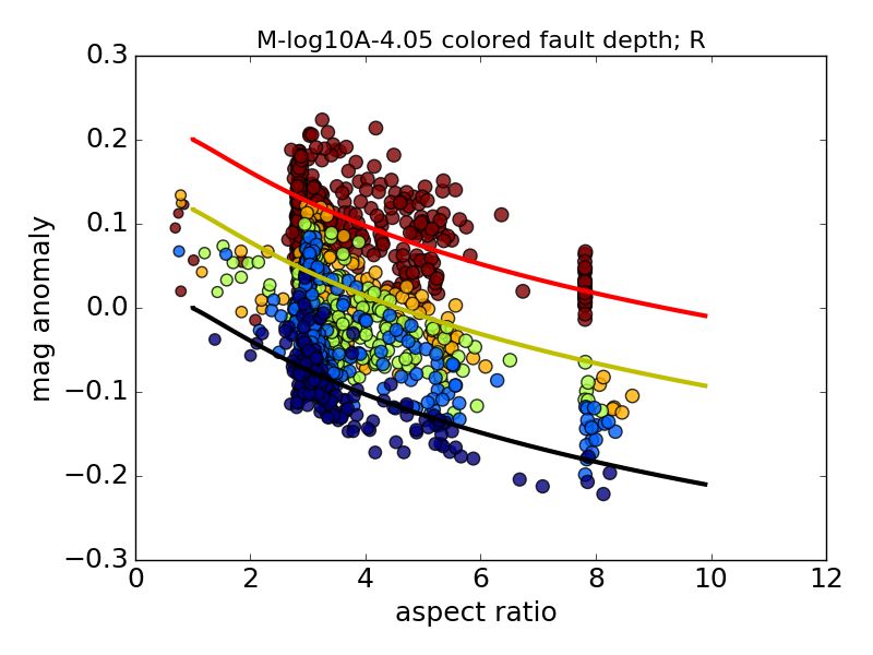

2

source physics of the simulator to improve the propagation velocity to obtain more realistic
directivity effects. These improvements, include: (1) Improving the accuracy of the stiffness
matrix by considering not just the finite area of the source patch, but the finite area of the
receiver patch as well. (2) Eliminating fixed sliding speed approximation during fast earth-
quake slip, and replacing it with slip velocity which is determined by the shear impedance
relationship. (3) Rather than instantaneous stressing rate updating, introducing a time
delay to stress rate updating on other elements which is motivated by a retarded green’s
function effect from finite wave speeds. An approximation of this effect uses a fixed delay
for all elements related to the source patch dimension, to maintain a minimum of updating
steps and preserve the fast algorithm. Together these source physics improvements lead to
improved propagation velocity.
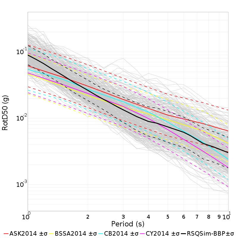
    Figure 2 shows spectra plots of an individual event, and an ensemble of events, compared
with empirical Ground Motion Models (GMMs). This gives an example of how the model
ground motions are calibrated and validated against empirical observations.
    Figure 3 shows an example of a full hazard curve calculated at a single site from the
full simulator catalog using a full 3D velocity model in Cybershake. This illustrates a fully
deterministic calculation of PSHA using the deterministic sequence of events and source
motions from the siumlator, with no stochastic aspects.

Figure 1: Propagation velocity as a function of patch hypocentral distance for four different
RSQSim parameterizations, each of which incorporates a new feature over the previous model.
The base model is the catalog used in Shaw et al. (2018), plotted with a dashed line. The first
modification, plotted with a dotted line, adds a new finite receiver patch capability to the stiffness
matrix calculations. The second modification, plotted with a dotted and dashed line, adds variable
slip speed capabilities to RSQSim with stepwise updating of sliding velocity on a patch during
earthquake slip. The final model, plotted with a solid line and used for PSHA calculations in this
study, also includes a time-delay to the static-elastic interaction. From [Milner, Shaw, et al.,
2020].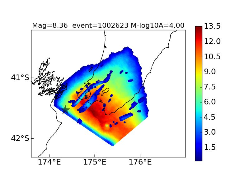

3

     (a)                                         (b)
Figure 2: Example ground motions from simulator events compared with Ground Motion Models
(GMM). RotD50 spectra for site USC from ruptures on the Mojave section of the San Andreas
Fault, computed with a one-dimensional (1D) velocity structure with VS30=500 m/s in the South-
ern California Earthquake Center (SCEC) BroadBand Platform (BBP). (a) Spectrum for a M 7.48
rupture on the Mojave section of the San Andreas Fault plotted as a thick black line. (b) Spectra
for 185 different 7.0 ≤ M ≤ 7.5 RSQSim ruptures on the Mojave section of the San Andreas Fault
simulated at USC plotted with thin gray lines, the mean of all 185 ruptures as a thick black line,
and the mean plus and minus one standard deviation with dashed black lines. GMM comparisons
(with plus and minus one standard deviation bounds marked with dashed lines) are plotted with
colored lines. GMM predictions are slightly different for (b) because distributions are averaged
across those predicted for each of the 185 RSQSim ruptures (rather than for a single M 7.48 rupture
in (a)). From [Milner, Shaw, et al., 2020].

Figure 3: Example of full deterministic PSHA calculation using 3D cybershake and simulator
ruptures, done at a single site. RSQSim simulation hazard curves at USC. CyberShake (3D) is
plotted with thick, black lines. (a) ASK2014 GMM comparisons curves in blue, with the complete
hazard curve plotted as a thick solid line. GMM curves computed from truncated log-normal
distributions at three-, two-, and one-sigma are plotted with dashed, dotted, and dotted and
dashed lines respectively. The 1D BBP hazard curve is included in yellow, and 95% confidence
bounds assuming a binomial distribution (representing sampling uncertainty from a finite catalog
duration) on the 3D simulated curve as a gray shaded region. From [Milner, Shaw, et al., 2020].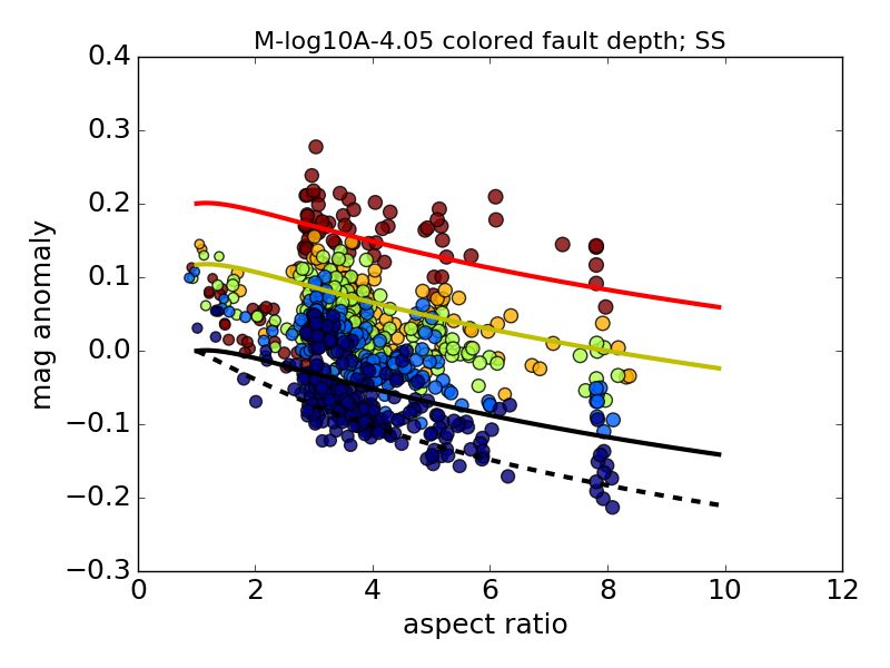

4

New Zealand simulator
”An Earthquake Simulator for New Zealand” (Shaw, et al., 2021)
    We present an earthquake simulator for New Zealand. It uses the RSQSim simulator
engine based on approximations of the rate-and-state friction equations. The full set of faults
considered in the most recent NZ national seismic hazard map are included in the simulator.
New simulator methods are introduced that allow for the inclusion and interaction between
upper plate faults and a subduction interface fault below them. The simulator generates
sequences of complex slip events and a catalog of finite ruptures hundreds of thousands
of years in length. Results from the simulator are evaluated through statistical testing
and comparison with geological and geophysical observations. These evaluations include a
spatial comparison against historical earthquakes, a comparison against rates of events in
the instrumental catalog, and a comparison against scaling relations. Significant aspects
of the resulting synthetic catalogue are discussed. These include substantial variability
over instrumental catalog timescales, and spontaneous ruptures which break both the upper
crustal faults and subduction interface co-seismically. A variety of potential uses of the
model are noted.
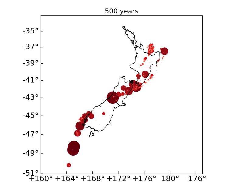
    Some figures illustrating the results are included below. Figure 4 shows epicenters in
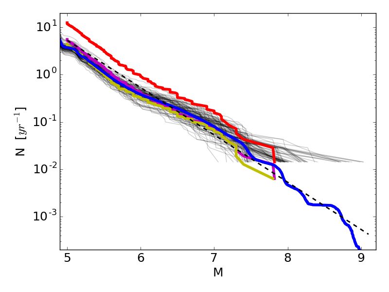
the model compared with historical and instrumental catalogs. Figure 5 shows distributions
of sizes of events in the model compared with the instrumental catalogs. Figure 6 shows
an example multifault event where the subduction interface breaks and faults in the upper
crustal plate break co-seismically. These events where the upper plate faults break co-
seismically with the subduction interface are very common in the model.

Scaling relations
(Shaw, 2021, in preparation) Further work was done on using earthquake simulators
to guide scaling relations. We have developed new magnitude-area scaling corrections valid
across all mechanisms which corrects for aspect ratio and burial and surface effects. This
scaling relation works well on the simulator ruptures. Figure 7 illustrates the dependence
on different burial depths, showing changes in magnitude anomalies (M− log10 A − C for
magnitude M and area A and constant C) as a function of aspect ratio and depth of buried
faults, for the case of a single fault. Figure 8 illustrates the fit of the new scaling relation
for a complex fault system, here the California UCERF3 faults.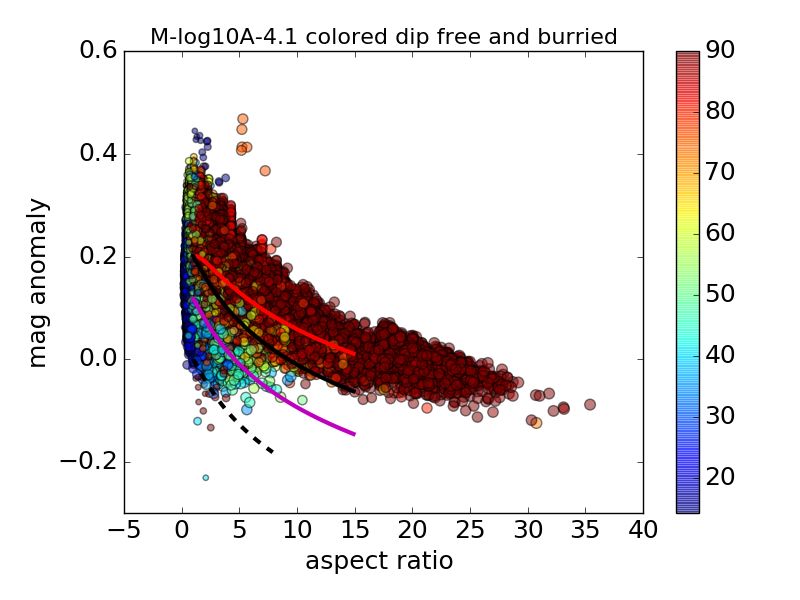

5

(a)                                                     (b)

                           (c)
      Figure 4: Epicenter map. Color and size coded by magnitude. Size scaled with area. Plotted
      sequentially in time, earlier smaller events may be hidden by later larger events. (a) Catalog length
      here is 5000 years. This is akin to long term catalog. (b) Catalog length 500 years. (c) Historical
      and instrumental catalog through 2020 of New Zealand earthquakes, compiled by GeoNet. Blue
      colormap highlights observed earthquakes. Only shallow (above 30km depth) events are plotted,
      since the model aims only to simulate shallow events. To first order we see spatial consistency.
      Some spatial differences in medium and large event productivity are seen in Central and Northern
      Hikurangi (in the East), with observed catalog being more productive. Also model catalog appears
      more productive in the Bay of Plenty (in the Northwest). From (Shaw et al., 2021).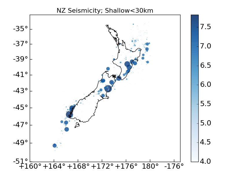

6

(a)                                                   (b)

(c)                                                   (d)
  Figure 5: Distribution of sizes of events. (a) Cumulative model events. Blue line is full model;
  green line is latitude restricted (< −41◦ ). (b) Differential model events. We see the cumulative
  distribution appearing fairly close to b = 1 here, though there are some underlying differences from
  that in the differential distribution. Dashed line shows b = 1, and has constant amplitude in all the
  plots to aid comparison between them. (c) Instrumental New Zealand seismicity 1940-2020. Red
  line is full catalog. Magenta line is reduced by a factor of 2/3 to represent anticipated on-fault rate,
  and an additional facotr of 2/3 for recalibration of magnitude estimates. Yellow line is restricted
  to exclude the last very active decade, covering the years 1940-2010. The blue line shows the
  mean model catalog from (a). In the background, grey lines show 100 different samples of model
  catalogs of 80 year lengths to show variability in productivity over the finite observational catalog
  timescale. The model is found to be consistent with the corrected catalog observations. (d) Test of
  model productivity with earthquake catalog when both are restricted to latitudes South of −41◦ ,
  excluding subduction zone area. Magenta line shows catalog from 1940-2020. Yellow line shows
  catalog restricted to years 1940-2010 omitting last decade with exceptionally high activity. Model
  mean with green line. Grey lines show 100 different samples of model catalogs of 80 year lengths
  to show variability in productivity. Again consistency of model and observations is found. From
  (Shaw et al., 2021).

7

      Figure 6: Map view of large M8.4 subduction event which also ruptures coseismically a number of
      upper plate faults. Main subduction fault is the Southern Hikurangi. The next largest participating
      faults by area are the Wellington, Wairarapa, and BooBoo faults, respectively. Color indicates slip
      in meters. The event initiates on the subduction interface at the epicenter indicated by the grey
      star. From (Shaw et al., 2021).

(a)                                                    (b)
      Figure 7: Single dipping fault magnitude anomalies for different depth ruptures. Different colors
      represent different depths of burried fault. Lines show scaling relation decreased anomaly with
      increasing depth of ruptures. (a) Strike Slip (b) Dip Slip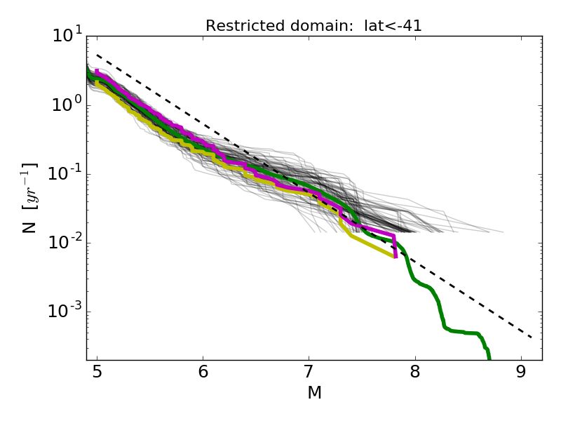

8

(a)                                                    (b)
      Figure 8: New magnitude area scaling with corrections for aspect ratio and buried rupture effects
      across different mechanisms. Points are events from RSQSim simulation of UCERF3 fault system.
      (a) Anomaly, difference between magnitude and log10 area as a function of aspect ratio. Points
      colored by dip. (b) Average over all events of residual as a function of lower magnitude cutoff
      once correction is applied. once correction is applied. Solid black line is mean absolute anomaly.
      Solid blue line is mean absolute residual. Dashed black line is mean absolute deviation of anomaly.
      Dashed blue line is mean absolute deviation of residual. Note the solid blue line is close to
      the dashed blue line, meaning there is little bias in the remaining residual. Note also the small
      remaining mean absolute residual, meaning we are on average capturing most of the systematic
      effects with the scaling corrections being applied. From [Shaw, in preparation, 2021].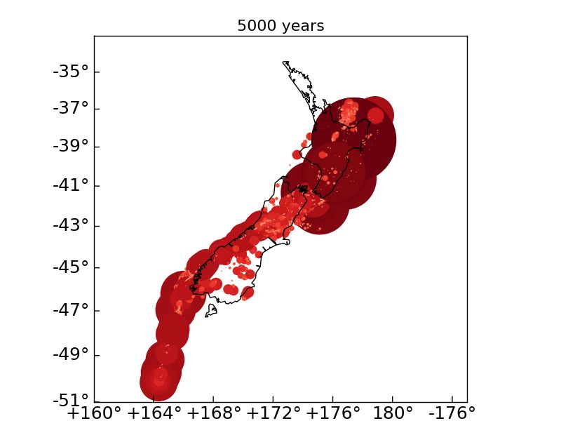

REFERENCES                                                                                 9

References
Milner, K. R., B. E. Shaw, C. A. Goulet, K. B. Richards-Dinger, S. Callaghan, T. H. Jordan,
 J. H. Dieterich, and E. H. Field, Toward Physics-Based Nonergodic PSHA: A Prototype
 Fully-Deterministic Seismic Hazard Model For Southern California, Bull. Seismol. Soc.
 Am., doi:10.1785/0120200216, 2021.
Shaw, B. E., K. R. Milner, E. H. Field, K. Richards-Dinger, J. J. Gilchrist, J. H. Dieterich,
  and T. H. Jordan, A physics-based earthquake simulator replicates seismic hazard statis-
  tics across California, Science Advances, 4, eaau0688, doi:10.1126/sciadv.aau0688, 2018.
Shaw, B. E., B. Fry, A. Nicol, and M. Gerstenberger, An earthquake simulator for New
  Zealand, p. preprint, 2021.