Regular Surfaces and Regular Maps (Non extended version)
←
→
Page content transcription
If your browser does not render page correctly, please read the page content below
Regular Surfaces and Regular Maps
                                   (Non extended version)

                                 Faniry Razafindrazaka, Konrad Polthier
                                         Freie Universität Berlin
                          {faniry.razafi,konrad.polthier}@fu-berlin.de

                                                          Abstract
      A regular surface is a closed genus g surface defined as the tubular neighbourhood of the edge graph of a regular
      map. A regular map is a family of disc type polygons glued together to form a 2-manifold which is flag transitive.
      The visualization of this highly symmetric surface is an intriguing and challenging problem. Unlike regular maps,
      regular surfaces can always be visualized as 3D embeddings. In this paper, we introduce an algorithm to visualize
      the regular surface of a regular map. Our algorithm takes as input the symmetry group of a regular map and output a
      3D realization of its regular surface. This surface can be interactively modified and used as a target shape for other
      regular maps. As a result, we find new realization of regular maps ranging from genus 9 to 85.

                                                     1    Introduction

A simple way to understand regular maps is to go back to the Platonic solids. They are the simplest examples
of regular maps. They are built from regular polygons, glued at their edges with an uniform vertex figure. Ad-
ditionally, they have the property of being flag transitive. In other words, moving a face or a vertex or an
edge to another face or vertex or edge preserves all adjacency properties. Regular maps also exist for high
genus surfaces. On the torus, they are checker-board, triangular and honeycomb like tilings. On surfaces of
genus g ≥ 2, they are tilings of the hyperbolic space. They were first described by Coxeter [3] and later on
enumerated by Conder [2] in the form of symmetry group.
     Lately, a lot of efforts have been made to visualize regular maps [10, 11, 6, 12, 8] but none of them
successfully find an automatic visualization procedure. Nevertheless, the work of van Wijk [6] is a huge
source of inspiration and serves as guidance to this paper. To tackle the hard problem of visualizing regular
maps, we go one step lower and define regular surfaces which were implicitly introduced in [6].
A regular surface is a closed genus g surface de-
fined as the tubular neighbourhood of the edge
graph of a regular map. It is proper to a regular
map. Unlike regular maps, regular surface can
always be visualized and we provide in this pa-
per all the ingredients to achieve that. In [6], a
regular surface is derived from an already em-
bedded regular map (in figure 1 are examples of
them). We relaxed this constraint by generating
directly the regular surface from the symmetry
group of the regular map.                                            Figure 1 : Regular surfaces (transparent)

     A regular map, following Conder [2], is denoted by Rg.i{p, q}, where g is the genus, i is a constant
and {p, q} is the Schläfi symbol of the tiling. The dual map is represented by Rg.i’{q, p}. In this paper, if
not explicitly stated, a regular map is denoted by G pq . The symmetry group is the same as in Conder [2]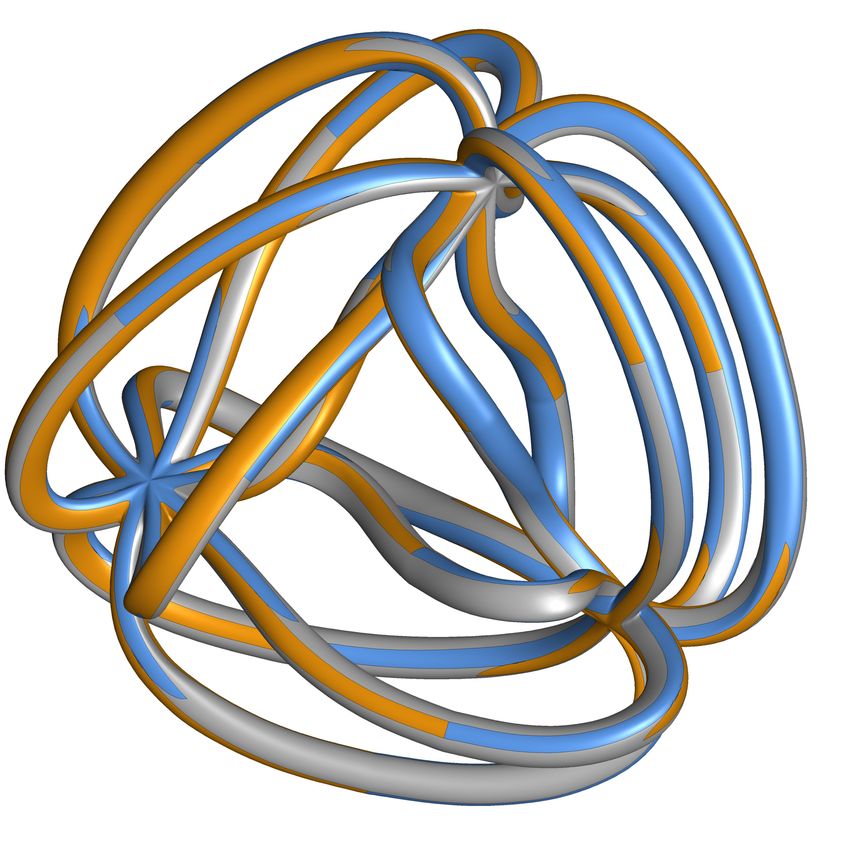
and is denoted by Sym(G pq ). We denote the regular surface of a regular map by Sg . We assume that the
reader is familiar with finitely generated groups, group action, surface topology and hyperbolic geometry.
For symmetry groups and group action, we use [3]; for surface topology, we use [5]; and for hyperbolic
geometry, we use [1, 9]. The remainings are basic notions of group theory.
Algorithm overview: the main steps of our algorithm are summarized as follow:

  1. Take a regular map G pq , defined by its symmetry group Sym(G pq ), as input.
     The list of all regular maps from genus 2 to 302, in the form of symmetry group, has been enumerated
     in [2].
  2. Enumerate all element representatives of Sym(G pq ) using advanced coset enumeration.
     This is done by using an advaced coset enumerator due to Havas G. and Ramsay C. [4].
  3. Make a hyperbolic realization of Sym(G pq ) and find the correct identifications at the boundary.
     Planar realization of regular maps are already understood and can be found in [6, 7, 8]. Finding the
     correct identification at the boundary, on the other hand, was not yet discussed. We give a detailed
     description in section 2.
  4. Take the edge graph of the realization and identify the edges at the boundary.
     This makes the edge graph consistent and induces unfortunately a degenerated regular surface.
  5. Define normals along the edge graph and apply a constrained physically based relaxation.
     Normals define the torsion of the regular surface Sg and should be preserved. We use the physically
     based relaxation procedure in [7, 8] to get smoothness and symmetry.
  6. (Optional) Introduce a group structure on Sg and find matchings with other regular maps G0pq using
     heuristics from [6].
  7. (Optional) Visualize G0pq .

    Points 3 to 5 are the most important steps of our algorithm. To understand them, we need to understand
how symmetry groups act on a geometry and what are the possible geometric realization of them.
      In section 2, we are going to construct a topological representation of G pq . This is realized in the
Poincaré model of hyperbolic space. In section 3, we explain briefly our identification algorithm which is
the first step to construct the medial axis of Sg . And finally, in section 5, we use our algorithm to generate
space models of regular maps. We call it targetless realization of regular maps because, unlike van Wijk’s [6]
cascade of mappings, our method does not need an actual 3D realization of the target regular map. Our space
of solution is then larger.

                   2    Topological Representation of High Genus Regular Maps

Let G pq be a regular map of genus ≥ 2 whose symmetry group
is given by Sym(G pq ) = hR, S, T | R(R, S, T )i. This group acts                    M0

transitively on a fundamental hyperbolic triangle M0 N0 O0 with               T            R
corner angles (π/p, π/q, π/2) setting R to be the rotation of an-       S
                                                                                  I RT
                                                                              N0     O0
gle 2π/p around M0 , S the rotation of angle 2π/q around N0 and
                                                                                  −1
                                                                                 S T RS
T the reflection across the edge M0 N0 (see figure 2). The re-
sulting triangular tiling group is denoted by Tri(G pq ). Each ele-
ment of Tri(G pq ) is a geometrical representation of an element of
Sym(G pq ). We denote by I the identity of Tri(G pq ).              Figure 2 : Tri(G pq ) and Line(G pq )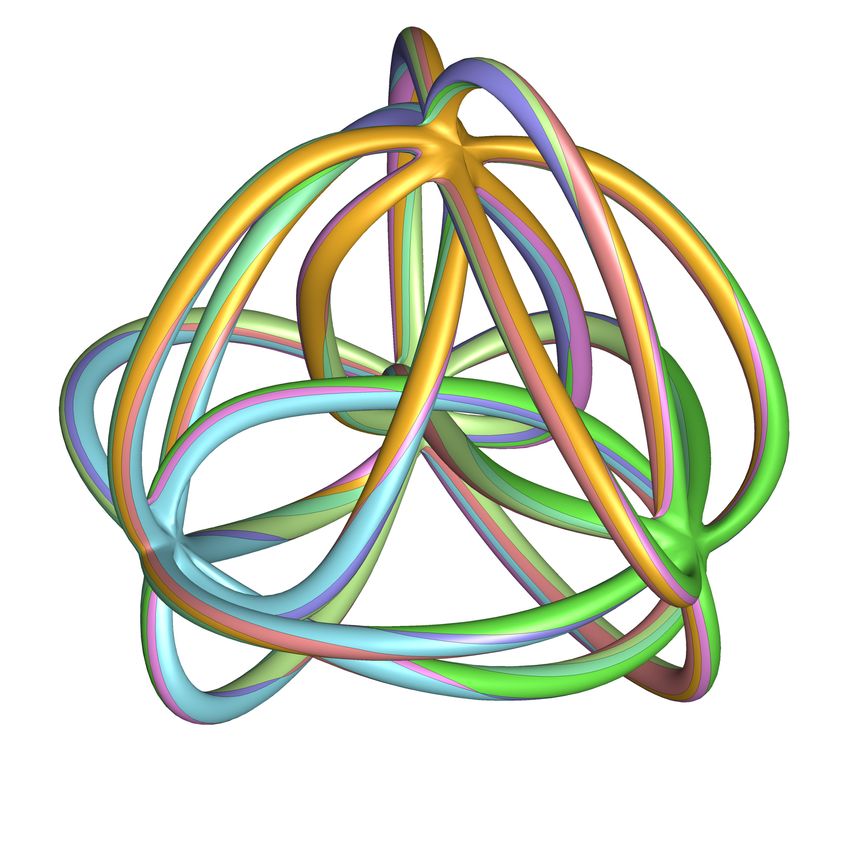
The correct identification at the boundary is obtained by finding the missing neighbour of each triangle
of Tri(G pq ) in Sym(G pq ) using the coset table. For example, in figure 3.a, triangle T does not have a neigh-
bour in Tri(G pq ) which in this case should be S. The coset table of Sym(G pq ) shows that S and S−1 R3 are
in the same equivalence class. Since a triangle corresponding to S−1 R3 exists in Tri(G pq ), we identify their
NO edges. We proceed in the same way for all boundary triangles. Figure 3.b is an example of a topological
representation of the regular map R2.4{5, 10} preserving flag transitivity.

                                                                                         2   1
                                      R2 T
                                 R3
                          R3 T               R2

                     R4                           R2 T
                                                                                 3                 0
                    T                              R
                          I                  RT

                          S−1 T          S−1 R4

                    S−1                             S−1 R3 T
                                                                                     0             3
                    S−1 RT
                                                  S−1 R3
                        S−1 R −1 2      S−1 R2 T
                             S R T
                                 S−1 R2                                                  1   2

                           (a)                                                   (b)
     Figure 3 : Representation of Sym(R2.4) in the hyperbolic space: (a) without identification and (b)
     with correct identifications.

     Each triangle of Tri(G pq ) has a corner vertex Mi Ni Oi obtained from M0 N0 O0 by the group action. The
set of all Ni Oi segments forms a line group Line(G pq ). This group is represented by red dotted segments and
blue segments in figure 3. In the topological representation, the boundary arrows show where a triangle or a
NO segment should be glued. We can use this information to make sure that an element L ∈ Line(G pq ) has
the same geometrical position as LS−1 T . Once all the L and LS−1 T have the same geometrical position, we
can generate the regular surface by associating to each NO segment a quarter-tube, similar to [6].

                                                       3   Boundary Identification

The goal of this section is to give the elements L and LS−1 T ∈ Line(G pq ) the same geometrical position. We
do this by using the identifications induced from Tri(G pq ). As already stated in the previous section, only the
segments of Line(G pq ) on the boundary triangle of Tri(G pq ) need to be moved. This is possible for Line(G pq )
but unfortunately not for Tri(G pq ).
      Suppose, for example, that we want to identify a directed edge a with edge b. Define the tail of a to
be ta and tb the one of b. Find all segments of Line(G pq ) having ta as endpoint and move these vertices at
the tail tb of b. In this process, only the endpoints of a is moved. We do the same for the head ha of a to the
head hb of b. Once both head and tail are matched, we update the geometrical position of a to be the one of
b. We iterate this process until all the boundary NO segments of Line(G pq ) are identified. In Figure 4 is an
illustration of the overall process applied to Line(R2.4).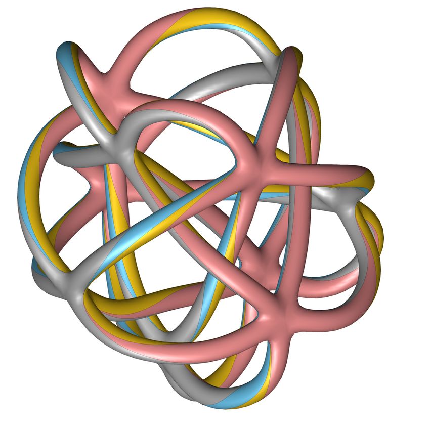
The input of our identification algorithm is Line(G pq ) and the output is again Line(G pq ) but the elements
L and LS−1 T have the same geometrical positions. In state 1 of figure 4, only four elements of Line(G pq )
are pairwise at the the same geometrical positions. The rest needs to be moved according to the glueing
procedure defined previously. The orange semi-dots represent the edges to be identified. The red dots
represent edges to be removed or updated. At state 10, there is only one step to be done since the curve 3 is
a loop.
     The identification does not depend on the order of the gluing. The resulting curves and loops are the
same. The only problem happens at the end of the identification where the ordering of the segments at the
nodes is ill defined. If we try to derive the regular surface, it might result in a degenerate tubular surface (see
figure 5). We solve this ambiguity in the next paragraph.

                                                                          2                                 2       1
                                                                                  1                                                             2           1
                              2           1

                                                                  3                       0           3                     0           3                       0
                  3                               0

                                                               0                              3       0                     3                                   3
                  0                               3

                              1           2                               1   2                            1       2                            1           2

                  1. identify side 0                          2. connectivity to h0                   3. connectivity to t0         4. update and identify side 1

                                                                          2   1                             2      1                            2       1
                      2           1
                                                              3                           0           3                     0           3                       0
              3                                   0

                                                      3                                       3                                 3                                   3

                      1           2                                           2
                                                                      1                                            2                                    2

              5. connectivity to h1                           6. connectivity to t1               7. update and identify side 2         8. connectivity to h2

                          2                                                                                 2
                                              1                                                                         1
              3                                                           2                           3                                             2
                                                  0                                   1                                     0
                                                                                                                                                                    1
                                                              3
                                                                                          0

                                                  3                                                                             3
                                                                                                                                            3
                                                                                              3
                                                                                                                                                                0
                                      2

               9. connectivity to t2                      10. update and identify side 3              11. update h3 and t3            12. connected Line(MT )
     Figure 4 : The process of identifying all elements L ∈ Line(MT ) to have the same geometrical
     positions as LS−1 T and vice versa. On the final shape, each green and blue line in state 1 are
     pairwise identified.

                                                          4    Construction of the Regular Surface

The regular surface obtained by the tubification of the edge graph of a regular map G pq is also a geometric
realization of Sym(G pq ). It is derived by associating to each element L ∈ Line(MT ) a quarter-tube QL . The
folding of the quarter tubes (left or right) depends on the corresponding element in Sym(G pq ). If the element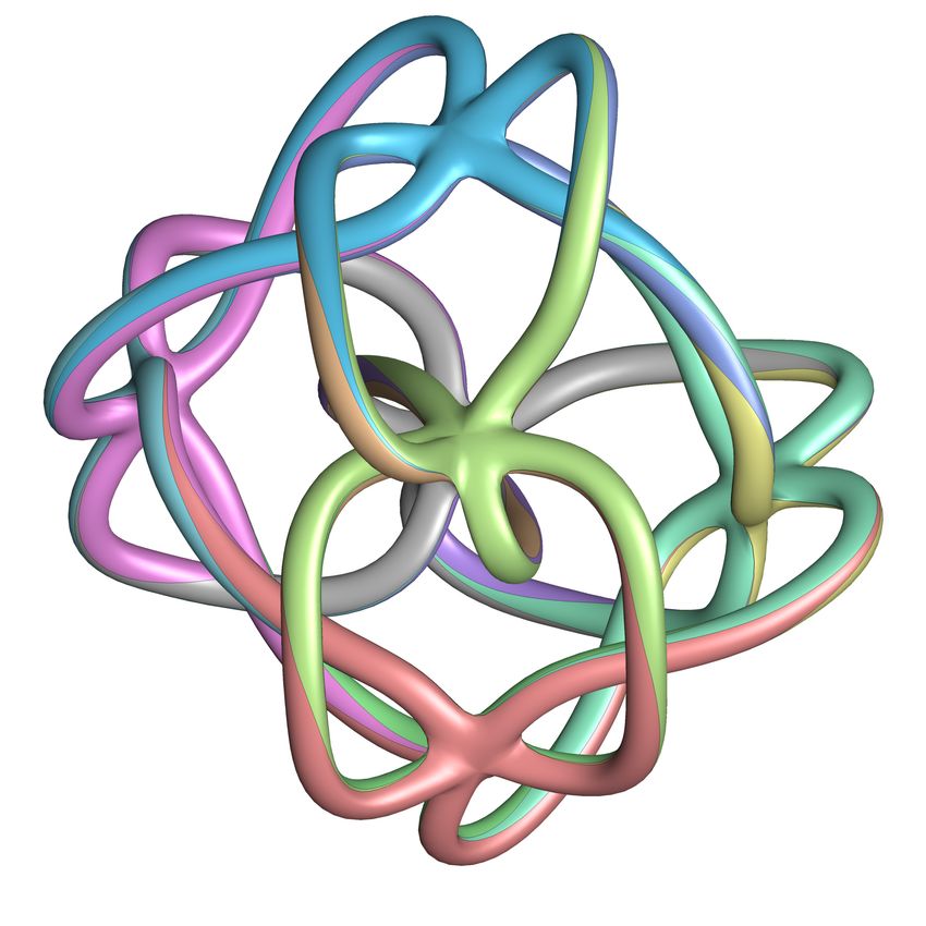
contains T (continuous segment in Line(G pq )), then it is folded left. Otherwise, it is folded right. The geo-
metrical construction of the quarter-tubes are described in [6, 7]. We call the resulting group Tub(G pq ). For
all QL ∈ Tub(G pq ), QL and QLS−1 T form a half tube. This is possible due to the identification done previously.
To have correct tube junctions at the nodes of Line(G pq ), it is necessary to have, additionally, each quarter
tube QL adjacent to QLT . It is equivalent to having a local ordering of each segment of Line(G pq ) at the
nodes.
     The local ordering at each node is obtained from Sym(G pq ). Suppose that we are at a node v which
is contained in the segments L0 , . . . , L2q−1 ∈ Line(MT ). The ordering of the segments, as in the hyperbolic
space, is reconstructed in a well defined plane at v. If L0 = L, then we must find a plane on which L1 =
LT, L2 = LS, . . . , L2q−2 = LSq−1 , and L2q−1 = LSq−1 T . In practice, this plane may not exist and degenerations
cannot be avoided (see, for example, figure 5 where there is no ordering at all). In our implementation, we
uses this information has a constraint and put Line(G pq ) in a string relaxation procedure. The result looks
better and respects the ordering of the tubes at the junctions (see figure 5.c). We did not write the relaxation
procedure in this paper, for more information, we refer to [7, 8].
      Figure 5.b is an example of such a plane where q = 4. The identification procedure does not guarantee
this orientation. Figure 5.c is an example of Line(G pq ) for which Tub(G pq ) does not have self-intersections
with a well defined tangent plane at the node.

                                                                L1 = LT

                                                     L2 = LS           L0 = L

                                              L3 = LST          v
                                                                      L7 = LS3 T
                                             L4   = LS2

                                                   L5 = LS2 T

                                                                L6 = LS3

                (a) Self intersection   (b) Correct neighbouring at a node (c) Correct tube junction
     Figure 5 : Wrong ordering at a junction may lead to a degeneration of the regular surface. The
     correct ordering is found on a suitable tangent plane.

                             5    Targetless Visualization of Regular Maps

Unlike regular maps, regular surface can always be visualized. One weak point of van Wijk’s approach [6]
is that the embedding of a regular surface depends on the embedding of the corresponding regular map. For
example, the regular surface of the map R2.5{5, 10} can be used as a space model of the map R5.8{4, 20}
but if R2.5 is not embedded, so is R5.8. Our algorithm handles this case and depends only on the regular
surface of the target map, not the target map itself. In figure 6 is our embedding of R5.8 together with its
dual.

              Figure 6 : A realization of the regular map R5.8{4, 20} (left) and its dual (right).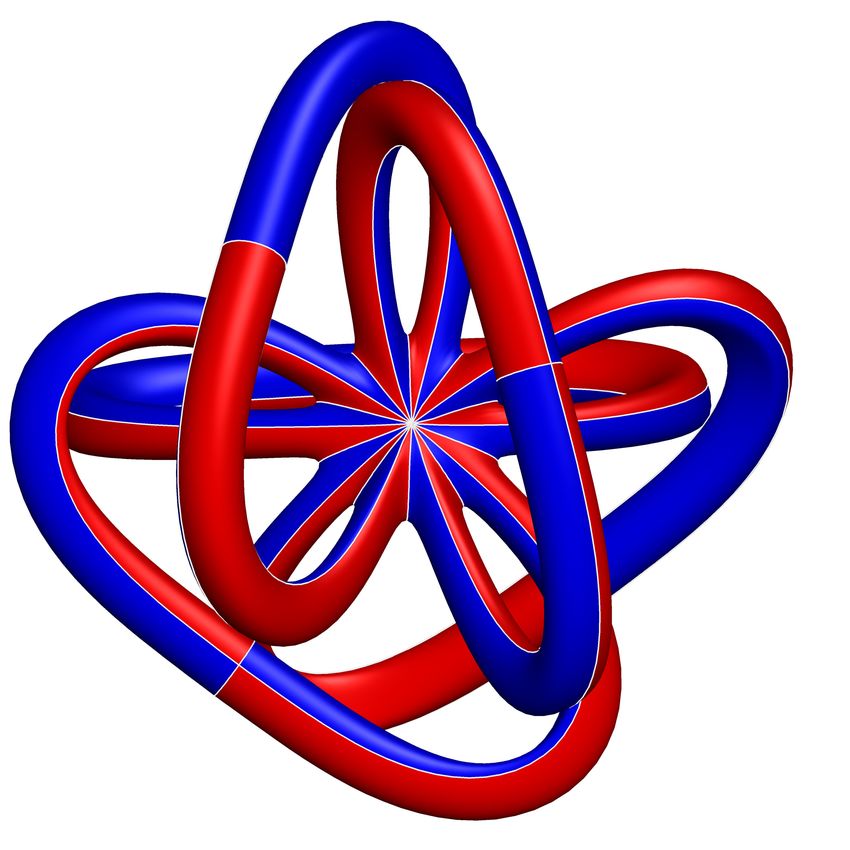
We find new realization of regular maps by combining van Wijk’s heuristic [6] with our algorithm. For
the purpose of visualization, we show regular maps for which p and q do not differ so much and regular
surfaces whose number of junctions are not 2 (hosohedral surfaces). We are not showing all the regular maps
we have found so far (more than 50 new cases), but rather emphasizing on the aesthetic visualization of few
realizations in our most symmetric realization
Our algorithm does not have a limitation as long as the matchings between the regular maps are pro-
vided. Van Wijk’s heuristic gives correct matchings of hundreds of regular maps which can all now be
visualized using our technique.
In this paper, we showed how to generate an embedding of a regular surface implicitly from a regular
map. The regular map itself does not have a priori an embedding. Hence, those maps (for example, R2.5) are
not handled by our algorithm. An interesting problem will be to find a similar procedure to realize directly
regular maps.
R9.3’ → R2.1’ (32 hexagons) R9.6’ → R3.5’ (16 octagons)
R9.13’ → R4.10 (2 16-gons) R9.17’ → R3.3’ (16 hexagons)
Figure 7 : Some regular maps of genus 9 in our most symmetric visualization.
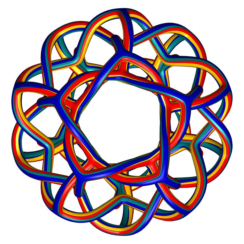
In figure 7 are four examples of genus 9 regular maps. R9.3’ has been already found by van Wijk in [6]
but we show here a better embedding with 3-fold symmetry. R9.13’ has only one junction with 18 incident
tubes. It was really hard to obtain this spiral shape like embedding.
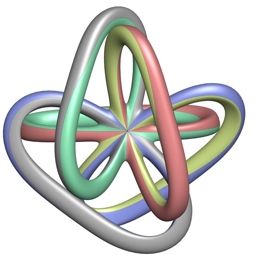
In figure 8 are six examples of larger genus regular maps. We particularly appreciate R13.3’ and R21.3’.
R13.3’ has 6 junctions with an octahedral symmetry and R21.3’ has an amazing full dodecahedral symmetry.
The later has 40 junctions placed on a double covered dodecahedron whose branch points are the center of
the faces. This suggests that a “polytopal” realization of the regular map R5.2’ (target map of R21.3’) is a
double covering of the dodecahedron.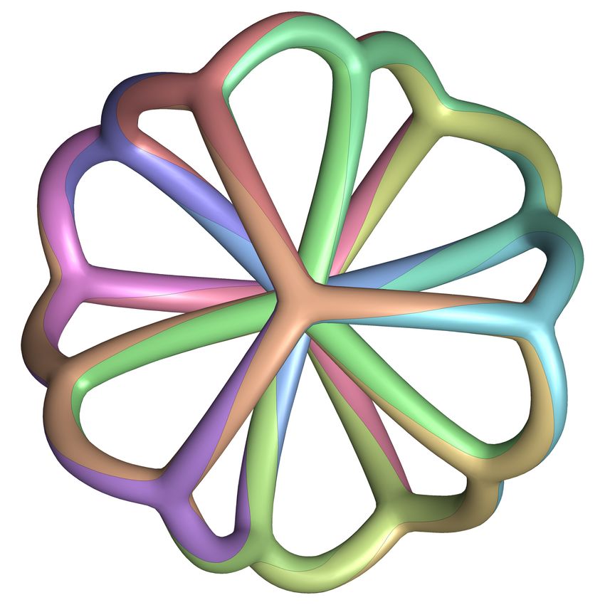
R13.1’ → R6.10’ (36 decagons)                  R13.3’ → R4.8 (12 dodecagons)

                R15.5’ → R6.9 (8 18-gons)                     R16.3’ → R6.6’ (20 decagons)

              R21.3’ → R5.2’ (80 hexagons)               R25.8’ → R10.16’ (24 dodecagons)
         Figure 8 : Some regular maps ranging from 13 to 25 in our most symmetric visualization.

     In figure 9 are three “really” large genus regular maps generated by our method. For these class of
regular maps, obtaining symmetry is a huge amount of work. Even a non self-intersecting surface is hard to
obtain. However, we believe that a careful understanding of the tubes and tiles can improve the symmetry of
the shape. R85.8’ is the regular map with the highest genus ever visualized so far (excluding the hosohedral
type of surfaces). We are particularly intrigued by its complex topology.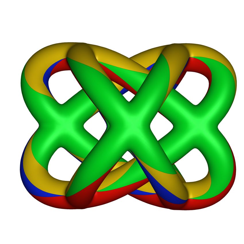
R41.3’ → R15.3’ (160 hexagons)      R61’.1 → R13.1’ (240 hexagons)      R85.8’ → R15.4’ (168 octagons)
                Figure 9 : Some large genus regular maps generated with intersection free.

Acknowledgement: We thank Jack van Wijk for his valuable suggestion. We also thank Ulrich Reitebuch
for suggesting the double covering of the dodecahedron for R21.3’. This research was supported by the
DFG-Collaborative Research Center, TRR109, Discretization in Geometry and Dynamics.

                                                References

 [1] Beardon A.F., The Geometry of Discrete Groups, Springer Verlag, New York, 1983.
 [2] Conder M,Regular Maps, August 2012,
     http://www.math.auckland.ac.nz/~conder/OrientableRegularMaps301.txt.
 [3] Coxeter H. and Moser W., Generators and Relations for Discrete Groups, Springer Verlag, 1957.
 [4] Havas G. and Ramsay C., ACE-Advanced Coset Enumerator, 2002,
     http://ww.itee.uq.edu.au/~cram/ce.html.
 [5] Massey W.S, A Basic Course in Algebraic Topology, Graduate Text in Mathematics, Springer-Verlag,
     1991.
 [6] van Wijk J. J., Symmetric Tiling of Closed Surfaces: Visualization of Regular Maps. Proc. SIGGRAPH
     2009, 49:1-12, 2009.
 [7] Razafindrazaka F., Visualization of High Genus Regular Maps, master’s thesis, Freie Universität Berlin,
     2012,
     http://page.mi.fu-berlin.de/faniry/files/faniry_masterThesis_2012.pdf.
 [8] Razafindrazaka F. and Polthier K., The 6-ring, In Proc. BRIDGES 2013 Conference, Entschede, Nether-
     lands, 279-286.
 [9] Reid M. and Szendro B, Geomery and Topology, Cambridge University Press, 2005.
[10] Séquin C. H., Patterns on the Genus-3 Klein quartic, In Proc. BRIDGES 2006 Conference, London,
     245-254.
[11] Séquin C. H., Symmetric Embedding of Locally Regular Hyperbolic Tilings, In Proc. BRIDGES 2007
     Conference, San Sebastian, 379-388.
[12] Séquin C. H., My Search for Symmetrical Embeddings of Regular Maps, In Proc. BRIDGES 2010
     Conference, Hungary, 85-94.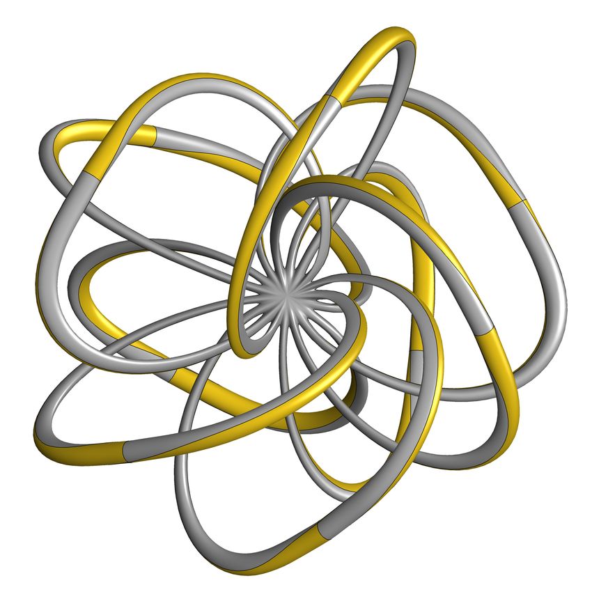
You can also read