Mobile Robots - Practicals - 716.034 2nd Laboratory Session Winter Term 2019/2020 - TU Graz

Mobile Robots - Practicals - 716.034
                2nd Laboratory Session
               Winter Term 2019/2020

      Prof. Gerald Steinbauer, Institute of Software Technology

Objective
The objective of this practical is that students gain experience in obtaining an
environment representation using onboard sensors. Students will learn how to
create a 2D gridmap using odometry and a range sensor. Moreover, the students
will work on globally consistent naps.

1       Introduction
Representing and understanding the environment is a fundamental capability
for an intelligent robot. Usually robots use an environment representation like
a map in various versions (geometric ot topological). In general such maps are
not available in advance and need to be obtained by the robot. This is the
mapping process. Due to the facts that sensor readings are uncertain and the
map usually cannot be directly obtained mapping is an estimation problem. In
particular mapping is an estimation problem with two interlinked estimation
problem. Thus, mapping is often named the Simultaneous Mapping and Local-
ization Problem (SLAM) because the position or path of the robot and the map
needs to be estimated simultaneously.
    In this laboratory session we will obtain a 2D gridmap using the robot’s
odometry and a laser range finder (lidar). A gridmap is a lattice structure of
random variables that represent the probability that a particular area of the
environment is occupied by an object like a wall. In order to ease the SLAM
problem we will follow the Mapping with Known Pose approach where we assume
an oracle that tells us the pose or path and estimate only the map.

2       Assignment
2.1     Setup
2.1.1    Robot
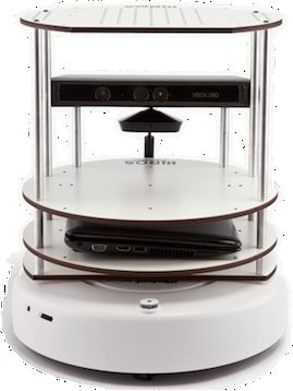
The robot used in this assignment is the Turtlebot 2 robot platform (see Figure
1). It is a differential drive robot based on the research version of the iRobot
Roomba vacuum cleaning robot (iRobot Create).
    The robot is fully supported by ROS and provides a lot of sensors:

                                       1

Figure 1: Turtlebot 2 Research and Education Platform.

   • wheel encoder/odometry
   • gyroscope
   • bumpers
   • cliff sensors
   • wheel drop sensor
   • infrared sensor for docking station
    The robot is usually equipped with a 3D visual sensor like the Microsoft
Kinect or the Asus Xtion. In the laboratory setting the robot is equipped with
a 2D laser range finder (lidar) from Hokuyo. The sensor is mounted at a hight
of 26 cm above the base point and 10 cm along the x-axis.
    The robot also provides 3 touch buttons on the back that can be used to
control the robot.
    The robot controller and the lidar are connected to the control laptop using
2 USB connections.
    The robot provides odometry information where the pose of the robot is
estimated using a sensor fusion of wheel encoders and a vertical gyroscope.

2.1.2   Software Framework
The software framework used for the assignment is based on the Robot Op-
eration System (ROS) [1]. The setup is tested for Ubuntu 16.04 and ROS
Kinetic. The setup is a catkinazied ROS package. The code is available
at https://git.ist.tugraz.at/courses/mobile_robots_public. ROS and
the package are already installed on a laptop that is paired with a robot.
    The setup comprises of basic driver packages for the Turtlebot
robot (http://wiki.ros.org/turtlebot bringup) and the Hokuyo lidar
(http://wiki.ros.org/urg node), and the own ROS node simple turtle. The
latter provides a C++ skeleton for implementing the mapping approach.
    In order to start the robot turn it on and use the command (in the command
line) roslaunch turtlebot bringup minimal.launch. If it works the robot
answers with a beep.

                                       2

To start the laser scanner driver use the command (in the command line)
roslaunch tug simple turtle laser.launch.
    In order to run the mapping node use the command (in the command line)
rosrun tug simple turtle simple turtle. Using the command in the com-
mand line) roslaunch kobuki keyop keyop.launch you are able to control
the robot using the keyboard.
    Using rviz you are able to visualize the different coordinate systems attached
to the robot and their changing if the robot is moved as well as the recorded
laser scan.

2.2    Task 1
The goal of the task is to implement mapping with known poses using odomery
information and distance data from the recorded laser scan.
    The basic estimation problem for a map m can be defined as:
    m∗ = arg maxP (m|u1 , z1 , u2 , z2 , · · · , ut−1 , zt−1 , ut , zt )
             m
where u represents the control inputs to the robot and z represents the recorded
measurements until time t.
    A grid map represents a 2 dimensional array of random variables the prob-
ability P (mi = occupied) that a cell mi is occupied by an object. Using the
assumption that the individual cells are independent we can reformulate the
map probability in the following      Q way:
    P (m|u1 , z1 , · · · , ut , zt ) = i P (mi |u1 , z1 , · · · , zt−1 , ut , zt )

    The probability P (mi = occupied) is dichotomous. So the probability can
be expressed using the log-odd ratio that avoids problems with rounding and
saturation and allows summation instead of multiplication when dealing with
factorization of probabilities:
    l(x) = log( PP(¬x
                  (x)           P (x)
                      ) = log( 1−P  (x )

    If we assume that we know the pose x of the robot we can reformulate the
map estimation problem as follows:
    P (mi |z1...t , x1...t )
Using the Markov assumption and the conditioned Bayes law we can reformulate
the estimation problem as follows:
    = P (mi |zPt(m
                 ,xt )P (zt |Xt )P (mi |zt−1 ,xt−t )
                    i )P (zt |z1...t−1 ,x1···t )
    This formulation represents a recursive Bayes Filter for the map estimation
problem. Given the probability of the map cell at time t − 1 as well as the
measurement zt and the pose xt at time t we can estimate the probability of
the map cell at time t.
We can formulate the same relation also for the counter probability:
    P (¬mi |z1...t , x1...t ) = P (¬miP|z(¬m     t ,xt )P (zt |Xt )P (¬mi |zt−1 ,xt−t )
                                                       i )P (zt |z1...t−1 ,x1···t )
Using the log-odd ratio we can represent the map probability by:
    l(mi |z1...t , x1...t ) = l(mi |zt , xt ) + l(mi |z1...t−1 , x1...t−1 ) − l(mi )
This formulation represents and update rule for the log-odd ratio representation
of a map cell. The first part represents the inverse sensor model that represents
the probability of a cell being occupied given a measurement and a pose). The
second part represents the log-odd ratio representation of the previous time.
The last part represents prior knowledge about the probability that a map cell

                                          3

is occupied. Usually this factor is zero as the probability of a cell being occupied
if no information is available is assumed to be 0.5 representing uncertainty about
the cell’s state.
    An important component is here the inverse sensor model that represents
the probability that a cell is occupied given a pose and a range measurement.
See Figure 2 for an example.

 Figure 2: Inverse Sensor Model for a Range Sensor. For the original see [2].

    The sensor model distinguish basically two areas. These are the area that
are inside the sensor cone (defined by the opening angle and maximum range)
and the area outside. For the outside area the sensor provides no information so
the probability is modeled by 0.5. Within the cone we distinguish three areas.
Until the measured distance that is caused by a reflection by an obstacle we can
assume that the probability for a cell being occupied is low. This is represented
by the valley in Figure 2. Usually the measurement uncertainty increases with
the response angle we see a smooth transformation of the probability towards
the uncovered area. For the area of the actual response we have a higher proba-
bility for the cell being occupied. Beyond the actual response we have again no
information about the status of the cell as sensors usually unable to look trough
obstacles. As before we have a smooth transition between probabilities in the
areas due to the uncertainties in the sensor characteristics.
    Given the inverse sensor model and the recursive filter formulation we are
able to integrate new sensor information in order to solve the map estimation
problem. Figure 3 depicts the update of a gridmap using one range measure-
ment.
    For     this     the    code    of   the    file   simple turtle.cpp       in
~/catkin ws mr/src/mobile robots public/tug simple turtle/src needs
to be modified. The skeleton holds the member occupancy grid map of type
Tug2dOccupancyGridMap. It represents a occupancy grid map with log-odd
ratio representation. It will be created with a given size (number of cells in
x and y direction), a cell size in meter (squared cells) and an offset for the
center of the map. It is basically organized as a double indexed array and can
be quired and updated in that way. Helper functions support the access using
real world coordinates. The node is organized in a way that it automatically

                                         4

Figure 3: Gridmap after the update with a range measurement. Black denotes
a most likely occupied cell. White denotes a most likely free cell. Gray denotes
a cell which is not conclusive. For the original see [2].

publishes the map in the background to be visualized in rviz.
    Every     time   new      laser    scan    is   received   the    callback
function                     void SimpleTurtle::laserScanCallback(const
sensor msgs::LaserScan::ConstPtr& msg) is triggered.              The sensor
message msg contains information about the sensor characteristics as well as
the actual measured laser scan. Based on the received laser scan you need to
update the gridmap. As oracle for the actual pose of the robot you can use the
odometry messages received by the node. Please consider in the map update
that a laser scan comprises several individual range measurements. In order to
implement an efficient update you need a kind of ray tracing along the sensor
beam. It is recommended to look into the Bresenham algorithm for drawing
lines in images.
    Once the code was modified the code needs to be compiled. The command
catkin make in the folder ~/catkin ws is doing the job. In order to activate
the changes the node needs to be restarted.
    Please use rviz to visualize the mapping process. Move the robot around
using the keyboard to map the entire laboratory. Please observe the reaction
of your implementation to measurement errors and dynamic changes in the
environment like moving obstacles or persons.

2.3    Task 2
To to the incremental approach to integrate sensor readings into the gridmap
and the uncertainty of the sensor readings it is possible that conflicting situations
like the one depicted in Figure 4 may appear. Due the conflict the open door
in a corridor is not represented in the map correctly.
    In order to improve this situation we can follow a global approach where
measurements are considered simultaneously in order to maximize the proba-
bilities of the obtained map given the sensor readings.
    We can reformulate the map estimation problem in the the following way:
    m∗ = arg maxP (m|u1 , z1 , u2 , z2 , · · · , ut−1 , zt−1 , ut , zt )
             m

                                         5

Figure 4: Conflicting gridmap after the update with two successive laser scans.
For the original see [2].

    m∗ = arg max P (z1...tP|m,x 1...t )P (m|x1...t )
                            (z1...t |x1...t )
               m
Given the independence of the individual cells, the fact that the prior of the map
is independent of the path the robot took and the fact that the denominator is
independent of the variable we maximize we can reformulate it in the following
way:           QT
    = arg maxη t=1 P (zt |m, xt )P (m)
           m
which can be reformulated using the logarithmic representation to the following
expression:          PT                       P
   = arg maxconst + t=1 logP (zt |m, xt ) + l0 i mi
           m
Which a fixed prior of P (mi ) = 0.5 we can focus on the first summation in the
maximization problem.
   To solve this maximization problem we can apply hill climbing approach on
the probability function. We start with an emptyPmap; mi = 0. As all cells are
                                                   T
independent we can maximize the term arg max t=1 logP (zt |xt , m with mi =
                                                       k=0,1
k) individually for each cell. We can flip individual cells from occupied to free
or vice versa if it improves the probability that all measurements are generate
by the underlying map with the flipped cell. We can repeat this for all cells and
stop if no improvement can be achieved anymore. As hill climbing is a greedy
search method we might end up in a local minima.

3     Lab Report
A written report about the work done in the lab and the results achieved needs
to be submitted by email to steinbauerist.tugraz.at by February 6 2020.
The subject is [mobile robots] 2nd laboratory session. Per student team
only one report needs to be submitted.
   The report needs to contain the name and identification number of all team
members. Moreover, for each task the report needs to contain:

                                                 6

• short description what you did to solve the given task
    • derivations, formulas and code snippets you used to solve the task - it
      needs to be comprehensive to let one understand your solution
    • drawings are always welcome and helpful
    • results achieved
    • short description of problems you faced in the lab including possible rea-
      sons and solutions

   The report needs to be submitted as PDF document with maximum of 6
pages.

4     Grading
The following points are awarded for the different tasks are listed in Table 1

                              Task       Points
                              Task 1       25
                              Task 2   10 (bonus)
                              Sum          35

                 Table 1: Grading: Achievable points per task.

References
[1] Robot Operating System (ROS). http://ros.org.
[2] Sebastian Thrun, Wolfram Burgard, and Dieter Fox. Probabilistic Robotics
    (Intelligent Robotics and Autonomous Agents). The MIT Press, 2005.

                                       7