The Art of Performance Tuning for CUDA and Manycore Architectures - David Tarjan (NVIDIA) Kevin Skadron (U. Virginia) Paulius Micikevicius (NVIDIA)
←
→
Page content transcription
If your browser does not render page correctly, please read the page content below
The Art of Performance Tuning for
    CUDA and Manycore Architectures

            David Tarjan (NVIDIA)
          Kevin Skadron (U. Virginia)
         Paulius Micikevicius (NVIDIA)

1
Outline
• Case study with an iterative solver (David)
– Successive layers of optimization
• Case study with stencil codes (Kevin)
– Trading off redundant computation against
bandwidth
• General optimization strategies and tips
(Paulius)Example of Porting an Iterative
Solver to CUDA
David Tarjan
(with thanks to Michael Boyer)
1MGVF Pseudo-code
MGVF = normalized sub-image gradient
do {
Compute the difference between each
element and its eight neighbors
Compute the regularized Heaviside
function across each matrix
Update MGVF matrix
Compute convergence criterion
} while (not converged)
2Naïve CUDA Implementation
250x
Speedup over MATLAB
200x
150x
100x
50x
2.0x 7.7x 0.8x
0x
C C + OpenMP Naïve CUDA
CUDA
• Kernel is called ~50,000 times per frame
• Amount of work per call is small
• Runtime dominated by CUDA overheads:
– Memory allocation
– Memory copying
3 – Kernel call overheadKernel Overhead
• Kernel calls are not cheap!
– Overhead of one kernel call: 9 μs
– Overhead of one CPU function: 3 ns
• Heaviside kernel:
– 27% of kernel runtime due to computation
– 73% of kernel runtime due to kernel overhead
4Lesson 1: Reduce Kernel Overhead
• Increase amount of work per kernel call
– Decrease total number of kernel calls
– Amortize overhead of each kernel call across
more computation
5Larger Kernel Implementation
MGVF = normalized sub-image gradient
do {
Compute the difference between each
pixel and its eight neighbors
Compute the regularized Heaviside
function across each matrix
Update MGVF matrix
Compute convergence criterion
} while (! converged)
6Larger Kernel Implementation
250x
Speedup over MATLAB
200x
150x
100x
50x
2.0x 7.7x 0.8x 6.3x
0x
C C + OpenMP Naïve CUDA Larger Kernel
CUDA
Memory Allocation 71%
Memory Copying 15%
Kernel Execution 9%
0% 20% 40% 60% 80% 100%
Percentage of Runtime
7Memory Allocation Overhead
10000
malloc (CPU memory) cudaMalloc (GPU memory)
1000
Time Per Call (microseconds)
100
10
1
0.1
0.01
1E-07 1E-06 1E-05 0.0001 0.001 0.01 0.1 1 10 100 1000
Megabytes Allocated Per Call
8Lesson 2:
Reduce Memory Management Overhead
• Reduce the number of memory allocations
– Allocate memory once and reuse it throughout
the application
– If memory size is not known a priori, estimate
and only re-allocate if estimate is too small
9Reduced Allocation Implementation
250x
Speedup over MATLAB
200x
150x
100x
50x 25.4x
2.0x 7.7x 0.8x 6.3x
0x
C C + OpenMP Naïve CUDA Larger Kernel Reduced
Allocation
CUDA
Memory Allocation 3%
Memory Copying 56%
Kernel Execution 31%
0% 20% 40% 60% 80% 100%
Percentage of Runtime
10Memory Transfer Overhead
1000
CPU to GPU GPU to CPU
100
Transfer Time (milliseconds)
10
1
0.1
0.01
0.001
1E-06 1E-05 0.0001 0.001 0.01 0.1 1 10 100 1000
Megabytes per Transfer
11Lesson 3:
Reduce Memory Transfer Overhead
• If the CPU operates on values produced by
the GPU:
– Move the operation to the GPU
– May improve performance even if the
operation itself is slower on the GPU
Memory Operation Memory
values Transfer (CPU) Transfer values
produced consumed
by GPU Operation by GPU
(GPU)
12 TimeGPU Reduction Implementation
MGVF = normalized sub-image gradient
do {
Compute the difference between each
pixel and its eight neighbors
Compute the regularized Heaviside
function across each matrix
Update MGVF matrix
Compute convergence criterion
} while (! converged)
13Kernel Overhead Revisited
• Overhead depends on calling pattern:
– One at a time (synchronous): 9 μs
– Back-to-back (asynchronous): 3 μs
Implicit Synchronization
Kernel Memory Kernel Memory Kernel
Synchronous:
Call Transfer Call Transfer Call
Asynchronous: Kernel Kernel Kernel Kernel Kernel
Call Call Call Call Call
14Lesson 1 Revisited:
Reduce Kernel Overhead
• Increase amount of work per kernel call
– Decrease total number of kernel calls
– Amortize overhead of each kernel call across
more computation
• Launch kernels back-to-back
– Kernel calls are asynchronous: avoid explicit or
implicit synchronization between kernel calls
– Overlap kernel execution on the GPU with
driver access on the CPU
15GPU Reduction Implementation
250x
Speedup over MATLAB
200x
150x
100x
60.7x
50x 25.4x
2.0x 7.7x 0.8x 6.3x
0x
C C + OpenMP Naïve CUDA Larger Kernel Reduced GPU
Allocation Reduction
CUDA
Memory Allocation 7%
Memory Copying 1%
Kernel Execution 80%
0% 20% 40% 60% 80% 100%
Percentage of Runtime
16Persistent Thread Block
MGVF = normalized sub-image gradient
do {
Compute the difference between each
pixel and its eight neighbors
Compute the regularized Heaviside
function across each matrix
Update MGVF matrix
Compute convergence criterion
} while (! converged)
17Persistent Thread Block
• Problem: need a global memory fence
– Multiple thread blocks compute the MGVF matrix
– Thread blocks cannot communicate with each other
– So each iteration requires a separate kernel call
• Solution: compute entire matrix in one thread
block
– Arbitrary number of iterations can be computed in a
single kernel call
18Persistent Thread Block: Example
MGVF Matrix MGVF Matrix
1 2 3 1 1 1
4 5 6 1 1 1
7 8 9 1 1 1
Canonical CUDA Approach Persistent Thread Block
(1-to-1 mapping between
threads and data elements)
19Persistent Thread Block: Example
GPU GPU
Cell Cell Cell Cell Cell Cell
SM SM SM SM SM SM
1 1 1 1 2 3
Cell Cell Cell Cell Cell Cell
SM SM SM SM SM SM
1 1 1 4 5 6
Cell Cell Cell Cell Cell Cell
SM SM SM SM SM SM
1 1 1 7 8 9
Canonical CUDA Approach Persistent Thread Block
(1-to-1 mapping between
threads and data elements)
20 SM = Streaming MultiprocessorLesson 4:
Avoid Global Memory Fences
• Confine dependent computations to a
single thread block
– Execute an iterative algorithm until
convergence in a single kernel call
– Only efficient if there are multiple independent
computations
21Persistent Thread Block
Implementation
250x
211.3x
Speedup over MATLAB
200x
150x
27x
100x
60.7x
50x 25.4x
2.0x 7.7x 0.8x 6.3x
0x
C C + OpenMP Naïve CUDA Larger Kernel Reduced GPU Persistent
Allocation Reduction Thread Block
CUDA
22Absolute Performance
25
Frames per Second (FPS)
21.6
20
15
10
5
0.11 0.22 0.83
0
MATLAB C C + OpenMP CUDA
23Conclusions
• CUDA overheads can be significant
bottlenecks
• CUDA provides enormous performance
improvements for leukocyte tracking
– 200x over MATLAB
– 27x over OpenMP
• Processing time reduced from >4.5 hours
toWhen Wasting Computation is a
Good Thing
Kevin Skadron
Dept. of Computer Science
University of Virginia
with material from
Jiayuan Meng, Ph.D. studentWhere is the Bottleneck?
• CPU
• CPU-GPU communication/coordination
• GPU memory bandwidth
• Maximize efficiency of memory transactions
• Traversal order, coalescing
• Maximize reuse
• Avoid repeated loading of same data (e.g. due to multiple iterations,
neighbor effects)
• Cache capacity/conflicts
• Important to consider the combined footprint of all threads
sharing a core
• Goldilocks tilesWhere is the Bottleneck, cont.
• Global synch costs
• Global barriers/fences are costly
• Block-sized tasks that can operate asynchronously—braided
parallelism—may be preferable to multi-block data parallelism
• Processor utilization
• Maximize occupancy, avoid idle threads
• This gives more latency hiding, but beware contention in the memory
hierarchy
• Avoid SIMD branch/latency divergence
• Minimize intra-thread-block barriers (__syncthreads)
• Match algorithm to architecture – work-efficient PRAM algorithms may
not be optimal
• Resource conflicts can limit utilization
• e.g., bank conflictsPrioritizing = Modeling
• Improving reuse may require more
computation – find optimum?
• Solution 1: Trial and error
• Solution 2: Profile, build a performance model
• Solution 3: Auto-tune
• Mainly useful for tuning variables within an
optimized algorithm, e.g. threads/block, words/load
• Costs of auto-tuning can outweigh benefitsIterative Stencil Algorithms
Ghost Zone Technique
                redundant execution
How accurate is it? • Performance at predicted trapezoid height no worse than 98% opt (ICS’09) • Then use auto-tuning to find the optimum
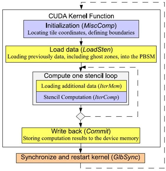
Establishing an analytical
   performance model
Computation vs. Communication
                                        • LoadSten: loading all
                                          input data for a trapezoid
                                          (including the ghost
                                          zone)
                                        • Commit: Storing the
                                          computed data into the
                                          global memory
                                        • MiscComp: Computation
                                          time spent in initialization
                                          (get thread and block
                                          index, calculate borders,
                                          etc)
                                        • IterComp: The major
                                          computation within
                                          iterations (assuming
   Normalized to trapezoid height = 1     mem. latency is 0)
                                        • GlbSync: Global
                                          synchronization, or
                                          kernel restart overhead
When to apply ghost zones? Lower dimensional stencil operations Narrower halo widths Smaller computation/communication ratio Larger tile size Longer synchronization latency
Summary

• Find bottlenecks
• Be willing to modify the algorithm
• Consider auto-tuning
Thank you!
Backup
Related Work
Redundant computation partition [L. Chen Z.-Q.
Zhang X.-B. Feng.]
Ghost zone + time skewing (static analysis) [S.
Krishnamoorthy et al.]
Optimal ghost zone size on message-passing grid
systems [M. Ripeanu, A. Iamnitchi, and I. Foster]
Adaptive optimization on grid systems [G. Allen et al.]
Data replication and distribution [S. Chatterjee, J.R.
Gilbert, and R. Schreiber][P. Lee]
Ghost zone on GPU [S. Che et al.]Experiments
Architecture parameters
Dynamic Programming
ODE solver
PDE solver
Cellular Automata
(Conway's Game of Life)
Benchmark parametersModel Validation Although the prediction error ranges from 2% to 30%, the performance model captures the overall scaling trend for all benchmarks.
How to optimize performance?
Gathering architecture parameters (once for
each architecture)
Profiling application parameters (small input
suffice, once for each application)
Calculate the optimal ghost zone size using
the analytical performance model
Adjust the code accordingly/Automatic code
generationTuning Kernel Performance
Paulius Micikevicius
NVIDIAKeys to Performance Tuning
• Know what limits your kernel performance
– Memory bandwidth
– Instruction throughput
– Latency
• Often when not hitting the memory or instruction
throughput limit
• Pick appropriate performance
– For example, Gflops/s not meaningful for
bandwidth-bound appsMemory Throughput
• Know the achievable peak
– Theoretical peak = clock rate * bus width
– About 75-80% is achievable in a memcopy
• Two ways to measure throughput
– App: bytes accessed by the app / elapsed time
– Hw: bytes moved across the bus / elapsed time
• Use Visual Profiler
• Keep in mind that total kernel (not just mem) time is used
• App and Hw throughputs can be different
– Due to access patterns
– Indicates how efficiently you are using the mem busOptimizing Memory-bound Kernels
• Large difference between app and hw throughputs
– Look to improve coalescing (coherent access by a warp, see
SC09 CUDA tutorial slides, CUDA Best Practices Guide for
more details)
– Check whether using texture or constant “memories” suits
your access pattern
• Consider “compression” when storing data
– For example, do arithmetic as fp32, but store as fp16
• Illustration: Mike Clark’s (Harvard) work on QCD (SC09 CUDA tutorial
slides)
• Consider resizing data tile per threadblock
– May reduce the percentage of bandwidth consumed by haloInstruction throughput
• Possible limiting factors:
– Raw HW instruction issue rate
– Serialization within warps, due to:
• Divergent conditionals
• Shared memory bank conflictsInstruction Issue Rate
• Know the kernel instruction mix
– fp32, fp64, int, mem, transcendentals
– These have different throughputs
– Could look at PTX (virtual assembly)
• Not the final optimized code
– Machine-language disassembler coming soon
• Know the hw throughput rates for various instruction types
– Programming guide / Best practices guide
• Visual Profiler reports instruction throughput
– Currently it’s the ratio:
(instructions issued ) / (fp32 instructions that could have been issued in the same elapsed time)
– Could go over 1.0 if dual-issue happens
– Currently not a good metric for fp64, or transcendental instruction-
bound codesSerialization
• One of:
– Smem bank conflicts, const mem bank conflicts
– Warp divergence
– A few others (much less frequent)
• Profiler reports serialization and divergence counts
• Impact on performance varies from kernel to kernel
• Assess impact before optimizing
– The below will give a perf estimate, but incorrect output
– Smem: change indexing to be either broadcasts or just
thread ID
– Divergence: change the condition to always take the same
path (try both paths to see what each costs)Latency
• Often the cause when neither memory nor
instruction throughput rates are close to the
peak rate
– Insufficient threads per multiprocessor to hide latency
• Consider grouping independent accesses by a thread
– Too few threadblocks when using many barriers per
kernel
• In these cases should aim at 3-4 concurrent threadblocks per
multiprocessor
• Fermi will have some performance counters to
help detectThreads per Multiprocessor and
Latency Hiding
• Memcopy kernel, one word per thread
• Quadro FX5800 GPU (102 GB/s theoretical)Another Perf Measurement Hack
• Separate and time kernel portions that access memory
and do “math”
– Easier for codes that don’t have data-dependent accesses or
arithmetic
• Comment out as much math as possible to get “memory-
only” kernel
• Comment out memory accesses to get “math-only” kernel
• Commenting reads is straightforward
• Can’t comment out writes = compiler will throw away “dead” code
• Put writes in an if-statement that always fails (but compiler can’t
figure that out)
• Comments also work well for assessing barrier
(__syncthreads) impact on performanceYou can also read