Ray-ONet: Efficient 3D Reconstruction From A Single RGB Image - arXiv
←
→
Page content transcription
If your browser does not render page correctly, please read the page content below
BIAN ET AL.: EFFICIENT 3D RECONSTRUCTION FROM A SINGLE RGB IMAGE                                                       1
arXiv:2107.01899v2 [cs.CV] 22 Oct 2021
               Ray-ONet: Efficient 3D Reconstruction
               From A Single RGB Image
               Wenjing Bian                                                              Active Vision Lab
               wenjing@robots.ox.ac.uk                                                   University of Oxford
               Zirui Wang                                                                Oxford, UK
               ryan@robots.ox.ac.uk
               Kejie Li
               kejie.li@eng.ox.ac.uk
               Victor Adrian Prisacariu
               victor@robots.ox.ac.uk

                                                                                               c) ONet           d) Ray-ONet
                                               a) Ray-ONet              b) Input image
                                                                                             0.333s per object    0.014s per object

               Figure 1: Ray-ONet recovers more details than ONet [16] while being 20× faster, by pre-
               dicting a series of occupancies õ along the ray that is back-projected from a 2D point p.

                                                                                 Abstract
                                             We propose Ray-ONet to reconstruct detailed 3D models from monocular images
                                         efficiently. By predicting a series of occupancy probabilities along a ray that is back-
                                         projected from a pixel in the camera coordinate, our method Ray-ONet improves the re-
                                         construction accuracy in comparison with Occupancy Networks (ONet), while reducing
                                         the network inference complexity to O(N 2 ). As a result, Ray-ONet achieves state-of-
                                         the-art performance on the ShapeNet benchmark with more than 20× speed-up at 1283
                                         resolution and maintains a similar memory footprint during inference. The project web-
                                         site is available at https://rayonet.active.vision.

               1                         Introduction
               3D reconstruction from a single view is an inherently ill-posed problem. However, it is triv-
               ial for a human to hallucinate a full 3D shape of a chair from a single image, since we have
               seen many different types of chairs from many angles in our daily life. Therefore, recover-
               ing a plausible 3D geometry from a single view is possible when enough prior knowledge
               is available, and in certain situations, might be the only feasible method when multi-view
               constraints are inaccessible, for instance, creating a 3D chair model from a chair image on a
               random website for an Augmented Reality (AR) application.
             © 2021. The copyright of this document resides with its authors.
             It may be distributed unchanged freely in print or electronic forms.
2          BIAN ET AL.: EFFICIENT 3D RECONSTRUCTION FROM A SINGLE RGB IMAGE

    Recently, the single-view object reconstruction field has been advanced significantly us-
ing deep learning. In particular, deep implicit representations, such as DeepSDF [18], Oc-
cupancy Networks [16] and their extensions [19, 23], demonstrate promising results on the
single-view 3D reconstruction task, by representing 3D shapes via a continuous function that
is embedded in network parameters. Although these methods enjoy the advantages of rep-
resenting 3D models in any resolutions and require small memory footprint and low storage
space, the inference speed is still an issue yet to address, as most existing methods require
querying millions of 3D locations to recover one 3D shape, leading to an O(N 3 ) complexity
when a simple 3D sampling strategy is employed.
    In this paper, we propose to predict a series of occupancies over 3D positions along a ray
back-projected from a query 2D location on an image plane given local and global image
features jointly. This formulation – viewer-centred ray-based occupancy prediction, taking
advantage of local and global image features – improves the reconstruction accuracy while
reducing the complexity to O(N 2 ).
    One issue of this viewer-centred reconstruction is the depth/scale ambiguity presented by
a single view (i.e., the same image can be rendered by a small object that is close to the cam-
era or a large object that is at a distance). A common practice is to normalise all ground-truth
shapes into a constant scale during training. However, this operation implicitly entangles the
shape learning with the scale ambiguity. Instead, we show how one can decouple these two
problems and improve the reconstruction accuracy by providing the network with a scale
calibration factor, which consists of a camera focal length and a camera-object distance.
    In summary, we introduce Ray-ONet with three contributions: First, our method predicts
a series of occupancies over 3D positions along a ray from a 2D query point, by condition-
ing an occupancy prediction function to both global and local image context, reducing the
complexity to O(N 2 ). Second, we introduce a scale calibration factor, to compensate for the
issue caused by different object scales. Third, we demonstrate on ShapeNet that our method
improves the overall 3D reconstruction accuracy while being 20× faster than ONet.

2    Related Work
Shape Representation. Computation efficiency and reconstruction quality are both effected
by the choice of representation for the model output. Researchers resort to volumetric repre-
sentations [5, 31] when deep networks are used for shape generation because 3D voxel grids
naturally fit into the convolutional operation. However, the resolution of voxels is often lim-
ited by memory, which grows exponentially for high-resolution outputs. Alternatively, point
clouds have been adopted [7], but they cannot represent surfaces directly. Meshes [29], being
compact and surface aware, assume a pre-defined topology.
    In recent years, implicit functions [4, 16, 18] are widely used for representing continuous
3D shapes. Networks using these implicit representations are trained such that the decision
boundary represents the iso-surface of an object shape. These models are able to reconstruct
high-resolution 3D shapes with low memory cost, but the inference time increases cubi-
cally with sampling resolution. Hybrid models [21, 22] which combine two representations
have also been developed recently. They couple explicit and implicit representations with
2 branches, where the explicit branch accelerates surface reconstruction while the implicit
branch reconstructs fine details of object shapes, but the network size is inevitably increased
dramatically. In contrast, Ray-ONet is able to speed up inference without increasing the
BIAN ET AL.: EFFICIENT 3D RECONSTRUCTION FROM A SINGLE RGB IMAGE                            3

memory footprint by predicting occupancy probability along a ray in a single network for-
ward.
Single-View 3D Reconstruction. Reconstructing from a single view is a severely ill-posed
problem, which was traditionally solved by “shape-from-X” techniques [12, 34] (X could
be silhouette, shading etc.) using geometric or photometric information. The resurgence of
deep learning in recognition tasks has encouraged researchers to solve single-view 3D recon-
struction in a data-driven manner. PSGN [7] and 3D-R2N2 [5] pioneer using a deep network
to learn a mapping from an RGB image to an object shape represented by voxels or point
clouds. Following works are able to achieve better performance by using more sophisticated
representations (e.g. Octree [27], dense point clouds [14], or implicit representations [16])
or building shape prior [30].
    More recently, CoReNet [20] predicts translation equivariant voxel grid using a variable
grid offset. It enables fast mesh extraction but still requires significantly more memory than
implicit models. The closest to our work is SeqXY2SeqZ [9], which also tries to reduce
the time complexity of inference in implicit representations. To this end, they design a
hybrid representation, which interpret a 3D voxel grid as a set of tubes along a certain axis.
However, its reconstruction resolution is fixed in all 3 dimensions, because of the built-in
location embedding matrices.
    Our work is also a hybrid approach, which explicitly predicts occupancy probabilities
along a certain ray that passes through a point on the input image. Unlike Han et al. [9],
we predict occupancies along a ray in a single network forward, which results in further
reduction in time complexity. In addition, the coordinate system of Ray-ONet is aligned
with the input image to take advantage of local features. As a result, we can predict 3D
shapes with fine details.
Coordinate System. Two types of coordinate systems are used in single-view object re-
construction: i) viewer-centred aligned to the input image or; ii) object-centred aligned to a
canonical position in the shape database. As discussed in [24, 28], an object-centred coor-
dinate system with aligned objects of the same category encourages learning category infor-
mation, which provides a robust prior for learnt categories, whereas predictions made in the
view space rely more on geometric information from the input image, and can generalise bet-
ter to unseen categories. Furthermore, recent works [20] using the viewer-centred coordinate
system demonstrate reconstruction with fine details by using image local feature. However,
they often assume 3D shapes are normalised to a constant scale. Instead, we introduce a
scale calibration factor to facilitate training given GT shapes in different scales.

3    Preliminary
Occupancy network (ONet) [16] formulates shape reconstruction as a continuous function
mapping problem, where the goal is to learn a function F that maps a 3D position x ∈ R3
to an occupancy probability õ, where {õ ∈ R : 0 < õ < 1}. The object shape is implicitly
represented by the decision boundary of the learned function F. To capture shape variations,
the occupancy function F above is often conditioned on observation, for example, an input
image. Mathematically, the occupancy prediction function F can be defined as:

                                        F(x, z) = õ,                                      (1)

where z is a latent code that encodes an input image I.
4           BIAN ET AL.: EFFICIENT 3D RECONSTRUCTION FROM A SINGLE RGB IMAGE

                        Encoder                               Occupancy
                                         Local Cont.           Decoder
                                           Mixer
      Cam
                       Ray-ONet

Figure 2: Ray-ONet Overview. Given an RGB image, Ray-ONet first maps the image to
a global feature descriptor z and a dense feature map C via an image encoder H. The local
feature Cp (feature at position p) and the position p, taken by the local context mixer J , are
mapped to a local context descriptor yp . Finally, the occupancy decoder D takes as input
yp , z and a scale factor s and predicts occupancies of 3D points along the back-projected ray
from position p.

    This mapping function, however, suffers from slow inference speed because the network
needs to query a large number of 3D positions to recover a high-resolution 3D reconstruc-
tion, which leads to O(N 3 ) complexity if the 3D positions are sampled in a regular 3D grid.
Although more sophisticated sampling strategies such as Multi-resolution IsoSurface Extrac-
tion (MISE) can be applied as in ONet [16], the inference speed is still largely restrained by
this query-every-3D-point strategy. This motivates us to develop a novel ray-based pipeline
that reduces the complexity to O(N 2 ).

4     Method
Given an input image I, we aim to build a 3D reconstruction in the camera space of I, instead
of in the canonical space as in ONet, by predicting series of occupancies along rays that are
back-projected for all image pixels.
    In other words, for each ray points to a 2D position p on the image plane, we predict
a series of occupancies along the ray behind the 2D position in one forward pass, hence
reducing the complexity to O(N 2 ). As a ray direction can be uniquely defined by the 2D
position p = (px , py ) in the viewer space, our Ray-ONet, which conditions the occupancy
prediction on the ray direction, can be considered as conditioned on the 2D position p. Fig. 2
presents an overview of our method.
    In the following sections, we first formalise our occupancy prediction function in Sec-
tion 4.1, followed by how we assemble it with image encoders and fusion modules (Sec-
tion 4.2) and a detail description of the scale calibration factor that facilitates training given
various scales of ground-truth object shapes (Section 4.3). Lastly, we describe our training
and inference pipeline in Section 4.4 and Section 4.5, including the training loss and the
mesh extracting process etc.

4.1    Occupancy Prediction
We now detail our occupancy prediction function. In Ray-ONet, we propose a function G:
                                         Local Global
                                        z}|{ z}|{
                                      G(p,Cp , z, s ) = õ,                                   (2)

which maps a 2D position p on an image I to a number of M occupancy estimations õ ∈ RM ,
conditioning on a global image feature z, a local image feature Cp and a scale calibration
BIAN ET AL.: EFFICIENT 3D RECONSTRUCTION FROM A SINGLE RGB IMAGE                                5

factor s. Technically, the occupancy prediction function G is parameterised by a Multi-Layer
Perceptron (MLP), and image global features z and local features Cp are encoded by a shared
CNN encoder. From now on, with a slight abuse of notation, we also refer G as our ray
occupancy network, as the network is just a parameterisation of the occupancy prediction
function.
    Comparing with the F(x, z) in the classical ONet in Eq. (1), which maps a 3D position x
to an occupancy estimation õ while conditioning on a global image feature, Ray-ONet uses
G(p,Cp , z, s) to map a 2D position p to a series of occupancy estimations õ by conditioning
the occupancy function on both local and global context. Ray-ONet, therefore, can predict
all M occupancies along a ray in a single network forward pass, reducing the complexity
to O(N 2 ). Moreover, as both our occupancy prediction function G and the classical F in
ONet are parameterised in a similar MLP structure, our method maintains a similar memory
footprint during inference.

4.2    Individual Modules
Given an input image I and its intrinsic and extrinsic camera parameters, we aim to extract
relevant information for the occupancy prediction function G. Specifically, we split the oc-
cupancy prediction function G to three modules: First, an image encoder H, which extracts
image global feature z and local feature Cp ; Second, a local context mixer J , which fuses
local image feature Cp with a ray that is defined by the 2D position p that it points to; and
Third, an occupancy decoder D, which decodes a series of occupancy estimations from both
local and global context.
Image Encoder H. We extract a global feature vector z and a feature map C from the input
image I using a ResNet-fashion CNN [10] H : I → (z,C). Specifically, the global latent code
z is an output of a ResNet-18, and the feature map C ∈ RH×W ×D is a result of concatenating
bilinear upsampled activations after the ResNet blocks, where H and W denote input image
resolution, and D denotes the feature dimension.
Local Context Mixer J . We parameterise the local context mixer module with an MLP
J : (Cp , p) → yp , which aggregates a 2D location p and an interpolated image feature Cp to
a fused local context feature yp .
Occupancy Decoder D. For a local feature yp at point p, we aim to predict a series of
occupancies, conditioning on a global feature z and a scale calibration factor s, via a decoder
D : (yp , z, s) → õ. Similar to ONet, we parameterise the decoder D in an MLP network with
skip links and Conditional Batch Normalisation (CBN).
    To summarise this section, we assemble the occupancy prediction network G with three
modules: an image encoder H, a local context mixer J and an occupancy decoder D:
                               Local Global
                             z}|{ z}|{
                           G(p,Cp , z, s ) = D(J (p,Cp ), z, s) = õ,                         (3)
where the global image feature z and the image feature map C are extracted the input image
I from encoder H.

4.3    Scale Calibration
The scale of the predictions is as important as the reconstructed shape because a correct
shape prediction but in a different scale to the ground truth can result in a large training loss.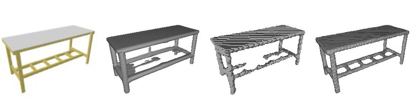
6             BIAN ET AL.: EFFICIENT 3D RECONSTRUCTION FROM A SINGLE RGB IMAGE
      Input       ONet       CoReNet      Ours       Input       ONet      CoReNet       Ours

Figure 3: Qualitative Reconstruction Results on ShapeNet. Note that Ray-ONet is able to
reconstruct fine details of object shapes, such as the complicated pattern on the chair back.
Instead of normalising all ground-truth shapes, we introduce the scale calibration factor s
as an extra dimension for the global feature to facilitate network training given ground-truth
shapes in different scales. Specifically, we define our scale calibration factor s = kck2 / f ,
where kck2 denotes the distance between a camera and a ground truth 3D model, and f
denotes the camera focal length.
    This scale calibration factor s conveys that the predicted shape scale should be propor-
tional to camera-object distance and inverse proportional to the camera focal length. In the
case of using a fixed focal length for the entire training set, the scale calibration factor can be
further reduced to kck2 . Note that this scale calibration factor is only needed during training.

4.4    Training
We use a binary cross-entropy loss L between predicted occupancies õ and ground truth
occupancies o to supervise the training of the encoder H, the mixer J and the decoder D:

                          L(õ, o) = −[o log(õ) + (1 − o) log(1 − õ)].                        (4)

    As we predict 3D models in the camera space of an input image, we rotate ground truth
3D models so that the projection of a ground truth 3D model on the input image plane
matches the observations on I. This step is necessary to acquire ground truth occupancies o
in the camera space of an input image.

4.5    Inference
During inference, as we do not have access to camera-object distance, nor camera intrinsics,
the scale calibration factor can be set to a random value in the range of the scaling factor
used during training. As a result, our method recovers correct shapes in an unknown scale
due to the inherent scale/depth ambiguity in the single-view 3D reconstruction task.
    Before extracting meshes using the Marching Cubes algorithm [15], we apply an addi-
tional re-sampling process on the Ray-ONet occupancy predictions, which is in the shape of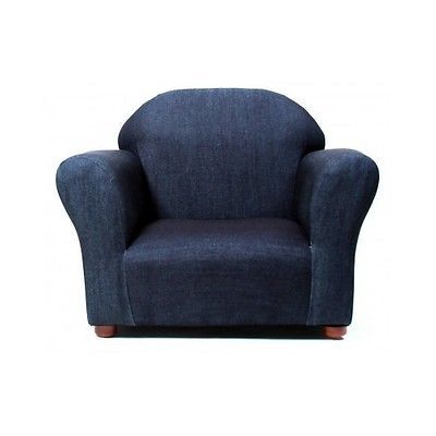
BIAN ET AL.: EFFICIENT 3D RECONSTRUCTION FROM A SINGLE RGB IMAGE 7
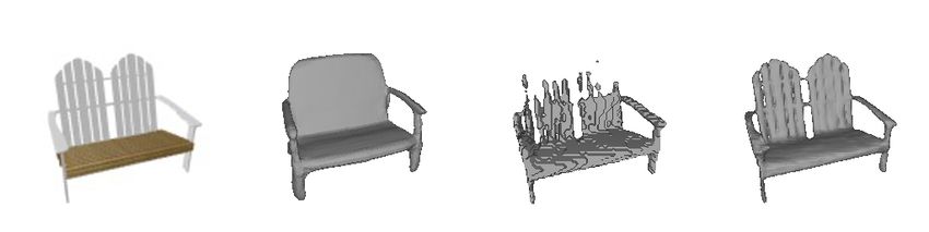
Input ONet ONet Ours Input ONet ONet Ours
Figure 4: Qualitative Reconstruction Results on Unseen Categories. We show Ray-ONet
can generalise better than our baselines on unseen categories, in which object shapes are
significantly different from the training classes (airplane, car, and chair).
a camera frustum due to the nature of our ray-based method, to get occupancies in a regular
3D grid. This re-sampling process can be simply done by trilinear interpolation.
5 Experiments
We conduct experiments to evaluate our method on two benchmarks, showing our method
achieves state-of-the-art performance while being much faster during inference. This section
is organised as follows, Section 5.1 reports the setup of our experiments. We compare our
reconstruction quality with baselines in Section 5.2. Memory and time consumption are
reported in Section 5.3. Lastly, we conduct an ablation study in Section 5.4.
5.1 Setup
Dataset. We evaluate Ray-ONet on the ShapeNet dataset [2], which is a large-scale dataset
containing 3D synthetic object meshes with category labels. To make fair comparisons with
prior works, we follow the evaluation protocol in ONet [16], taking a pre-processed subset
from 3D-R2N2 [5], which includes image renderings from 13 classes in ShapeNetCore v1
[2] and adopting the same train/test splits.
Metrics. Following ONet [16], we adopt the volumetric IoU, the Chamfer-L1 distance, and
the normal consistency score (NC) as the evaluation metrics. The volumetric IoU is evaluated
on 100k randomly sampled points from the bounding volume. Additionally, we compute IoU
on voxelised meshes in order to compare with some other baseline models. Methods with
different IoU evaluation methods are separately listed in Table 1. Excepting from Table 1,
our paper follows ONet’s IoU evaluation method by default.
Implementation Details. Network initialisation: Apart from the image encoder H, which
is fine tuned from an ImageNet[6]-pretrained ResNet-18 backbone[10] with a random ini-
tialised fully-connected layer head, the local context mixer J and the occupancy decoder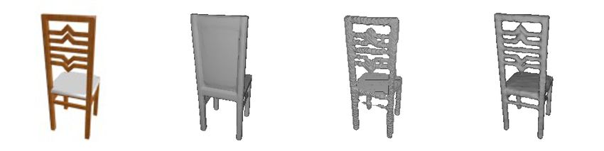
8              BIAN ET AL.: EFFICIENT 3D RECONSTRUCTION FROM A SINGLE RGB IMAGE

D are both trained from scratch. Training details: During training, we randomly sample
1024 pixels on an input image and predict occupancies for 128 points that are equally spaced
between a defined depth range on the rays. We use a batch size of 64, with an Adam[11] op-
timiser and a learning rate of 10−4 . Network architecture: A detailed description of network
architectures is available in the supplementary material.

5.2     Reconstruction Accuracy
Standard Reconstruction. We evaluate the performance of Ray-ONet on the standard
3D reconstruction task, training/testing on all 13 categories. We compare our model with
prior works including ONet [16], AtlasNet [8], CoReNet [20], DmifNet [13], 3D43D [1],
DISN [32] and Ladybird [33]. Note that ONet, AtlasNet, DmifNet and DISN are object-
centred models and the others are viewer-centred. DISN and Ladybird have different object
scale from ours, hence we only evaluate IoU, which is scale-invariant. Table 1 reports that
our model achieves state-of-the-art 3D reconstruction accuracy on the ShapeNet benchmark.

IoU ↑          airplane   bench   cabinet     car    chair   display    lamp   loudspeaker    rifle    sofa    table   telephone   vessel   mean
ONet            0.591     0.492    0.750    0.746   0.530     0.518    0.400      0.677      0.480    0.693   0.542      0.746     0.547    0.593
DmifNet         0.603     0.512    0.753    0.758   0.542     0.560    0.416      0.675      0.493    0.701   0.550      0.750     0.574    0.607
CoReNet†        0.543     0.431    0.715    0.718   0.512     0.557    0.430      0.686      0.589    0.686   0.527      0.714     0.562    0.590
3D43D           0.571     0.502    0.761    0.741   0.564     0.548    0.453      0.729      0.529    0.718   0.574      0.740     0.588    0.621
Ours            0.574     0.521    0.763    0.755   0.567     0.601    0.467      0.726      0.594    0.726   0.578      0.757     0.598    0.633
DISN            0.617     0.542    0.531    0.770   0.549     0.577    0.397      0.559      0.680    0.671   0.489      0.736     0.602    0.594
Ladybird        0.666     0.603    0.564    0.802   0.647     0.637    0.485      0.615      0.719    0.735   0.581      0.781     0.688    0.656
Ours            0.630     0.630   0.806     0.815   0.631    0.652     0.549      0.768      0.662    0.768   0.654      0.773     0.658    0.692
Chamfer-L1 ↓   airplane   bench   cabinet     car    chair   display    lamp   loudspeaker    rifle    sofa    table   telephone   vessel   mean
AtlasNet∗       0.104     0.138    0.175    0.141   0.209     0.198    0.305      0.245      0.115    0.177   0.190      0.128     0.151    0.175
ONet            0.134     0.150    0.153    0.149   0.206     0.258    0.368      0.266      0.143    0.181   0.182      0.127     0.201    0.194
DmifNet         0.131     0.141    0.149    0.142   0.203     0.220    0.351      0.263      0.135    0.181   0.173      0.124     0.189    0.185
CoReNet†        0.135     0.157    0.181    0.173   0.216     0.213    0.271      0.263      0.091    0.176   0.170      0.128     0.216    0.184
3D43D           0.096     0.112    0.119    0.122   0.193     0.166    0.561      0.229      0.248    0.125   0.146      0.107     0.175    0.184
Ours            0.121     0.124    0.140    0.145   0.178     0.183    0.238      0.204      0.094    0.151   0.140      0.109     0.163    0.153
NC ↑           airplane   bench   cabinet     car    chair   display    lamp   loudspeaker    rifle    sofa    table   telephone   vessel   mean
AtlasNet∗       0.836     0.779    0.850    0.836   0.791     0.858    0.694      0.825      0.725    0.840   0.832      0.923     0.756    0.811
ONet            0.845     0.814    0.884    0.852   0.829     0.857    0.751      0.842      0.783    0.867   0.860      0.939     0.797    0.840
DmifNet         0.853     0.821    0.885    0.857   0.835     0.872    0.758      0.847      0.781    0.873   0.868      0.936     0.808    0.846
CoReNet†        0.752     0.742    0.814    0.771   0.764     0.815    0.713      0.786      0.762    0.801   0.790      0.870     0.722    0.777
3D43D           0.825     0.809    0.886    0.844   0.832     0.883    0.766      0.868      0.798    0.875   0.864      0.935     0.799    0.845
Ours            0.830     0.828    0.881    0.849   0.844     0.883    0.780      0.866      0.837    0.881   0.873      0.929     0.815    0.854

Table 1: Reconstruction Accuracy on ShapeNet. We show Ray-ONet achieves state-of-
the-art reconstruction accuracy in all three evaluation metrics. For IoU evaluation, the first
group (5 rows) follows ONet’s evaluation pipeline, the second group (3 rows) follows DISN’s
pipeline. The notation ∗ denotes results taken from [16] and † denotes results we train their
public code and evaluate in ONet’s protocol. All other results are taken from corresponding
original publications.
Reconstruction on Unseen Categories. To evaluate the generalisation capability, we train
our model on 3 classes (airplane, car, and chair) and test on the remaining 10 classes. To
make a fair comparison, we additionally train an ONet model with the viewer-centred setup,
named ONetview . Table 2 reports that our model performs better than all baselines in this
setup.
5.3     Memory and Inference Time
As shown in Table 3, Ray-ONet is over 20× faster than ONet even if the efficient Multi-
resolution IsoSurface Extraction is used in ONet while maintaining a similar memory foot-
print. It is worth noting that 3D-R2N2 [5] uses a 3D auto-encoder architecture to predict on
the discretised voxel grid. Although it is 4× faster than Ray-ONet, it produces inferior re-
construction accuracy and requires a much larger memory size with 20× parameters. Since
BIAN ET AL.: EFFICIENT 3D RECONSTRUCTION FROM A SINGLE RGB IMAGE                                                        9

 IoU ↑          bench   cabinet   display   lamp    loudspeaker    rifle    sofa   table   telephone   vessel   mean
 ONet           0.251    0.400     0.165    0.147      0.394      0.172    0.505   0.222     0.147     0.374    0.278
 ONetview       0.241    0.442     0.204    0.135      0.449      0.104    0.524   0.264     0.239     0.302    0.290
 3D43D          0.302    0.502     0.243    0.223      0.507      0.236    0.559   0.313     0.271     0.401    0.356
 Ours           0.334    0.517     0.256    0.246      0.538      0.253    0.583   0.350     0.277     0.394    0.375
 Chamfer-L1 ↓   bench   cabinet   display   lamp    loudspeaker    rifle    sofa   table   telephone   vessel   mean
 ONet           0.515    0.504     1.306    1.775      0.635      0.913    0.412   0.629     0.659     0.392    0.774
 ONetview       0.443    0.418     0.840    2.976      0.496      1.188    0.343   0.470     0.532     0.469    0.818
 3D43D          0.357    0.529     1.389    1.997      0.744      0.707    0.421   0.583     0.996     0.521    0.824
 Ours           0.228    0.351     0.592    0.485      0.389      0.307    0.266   0.299     0.453     0.304    0.367
 NC ↑           bench   cabinet   display   lamp    loudspeaker    rifle    sofa   table   telephone   vessel   mean
 ONet           0.694    0.697     0.527    0.563      0.693      0.583    0.779   0.701     0.605     0.694    0.654
 ONetview       0.717    0.762     0.600    0.508      0.740      0.505    0.796   0.740     0.673     0.679    0.672
 3D43D          0.706    0.759     0.638    0.618      0.749      0.588    0.784   0.731     0.700     0.690    0.696
 Ours           0.736    0.762     0.640    0.642      0.762      0.609    0.806   0.764     0.670     0.703    0.709
Table 2: Reconstruction Accuracy on Unseen Categories. We report the performance of
different models on 10 unseen categories after trained on 3 categories. Our method outper-
forms all prior works in almost all categories.

SeqXY2SeqZ [9] has not released their code, we can only compare with them on complex-
ity and accuracy. The inference time complexity of SeqXY2SeqZ is O(N 2 ) × lRNN , where
lRNN denotes the number of the recurrent steps. While being more efficient, we outperform
SeqXY2SeqZ by 0.152 measured in IoU at 323 resolution (SeqXY2SeqZ reports its IoU at
this resolution).

                 Methods                            ONet     3D-R2N2         CoReNet        Ours
                 # Params (M)                        13.4     282.0            36.1         14.1
                 Inference Memory (MB)              1449       5113           2506          1559
                 Inference time (ms)                333.1       3.4            37.8         13.8
Table 3: Comparisons of Number of Parameters, Inference Memory and Inference
Time at 1283 Resolution. The inference time measures the network forward time only
and does not include any post-processing time.

5.4    Ablation Study
We analyse the effectiveness of the scale calibration factor s, the global and local image
features as well as the architecture design.
Effect of the Scale Calibration Factor. Training with the scale calibration factor can lead
to better reconstruction accuracy as reported in Table 4. This shows that decoupling scale
from shape learning not only enables us to train with varying scales of ground-truth shapes
but also helps in network convergence. As shown in Fig. 5, the scale factor helps to locate
the object and reconstruct the object with correct scale.
Effect of Global and Local Image Features. Both global and local image features are
important for reconstruction accuracy as suggested by the performance gap between w/ and
w/o features in Table 4. Visualisation in Fig. 5 shows that local feature enables more details
to be reconstructed, and global feature gives prior knowledge about object shape.
Effect of Architecture. We test a variation of our model by removing the Local Context
Mixer and concatenating all inputs (z, s,Cp , p) to feed into an Occupancy Decoder with
MLPs. The evaluation mIoU for this variation is 0.610, showing our original design can
achieve better performance.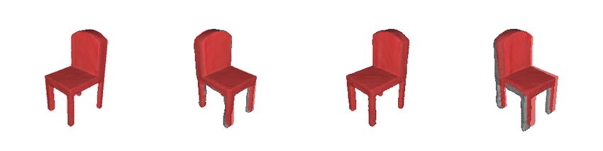
10             BIAN ET AL.: EFFICIENT 3D RECONSTRUCTION FROM A SINGLE RGB IMAGE
       Input              Ours                    w/o local                            w/o global

                          Ours                     w/o scale

Figure 5: Visualisation for Ablation Study. Without the local feature, details of the object
can not be recovered. Without the global feature, artifacts occur in other views. Without the
scale factor, the scale of prediction (grey) can be different from ground truth (red).
                                       IoU ↑ Chamfer-L1 ↓                    NC ↑
                      Ours             0.633       0.153                     0.854
                      w/o scale s      0.545       0.226                     0.818
                      w/o global z 0.574           0.206                     0.821
                      w/o local Cp 0.525           0.224                     0.802
Table 4: Ablation Study. We show the effectiveness of the                   scale calibration factor s, the
global image feature z and the local image feature Cp .
                                                                     0.64
5.5    Discussion                                                    0.62

We study the effect of changing number of samples          0.60
                                                               IoU

in the image-plane dimension S plane and along the         0.58
                                                                                  Image Plane
ray direction M. Results: Fig. 6 shows that although       0.56                   Ray Direction
the reconstruction quality relates to both sampling di-         32 64      128                256
mensions, having M > 128 along a ray cannot fur-            Number of Samples along Each Dimension
ther improve reconstruction quality, whereas sam-
pling more pixels in an image plane is still beneficial. Figure 6: IoU of various No. of sam-
Insights: These results are not surprising as deducing ples on a ray and in an image plane.
occluded space is an ill-posed problem and can only be resolved from learning shape priors
during training, which is bottlnecked by training data rather than M = 128. On the other
hand, since sampling more pixels in an image plane provides richer texture details, the re-
construction quality improves when S plane increases. Setup: To study the effect of different
S plane , we fix M = 128 and test with S plane = 322 |642 |1282 |2562 . To study the effect of
different M, we fix S plane = 1282 and test with M = 32|64|128|256.

6     Conclusion
We proposed Ray-ONet, a deep neural network that reconstructs detailed object shapes ef-
ficiently given a single RGB image. We demonstrate that predicting a series of occupancies
along back-projected rays from both global and local features can significantly reduce the
time complexity at inference while improving the reconstruction quality. Experiments show
that Ray-ONet is able to achieve state-of-the-art performance for both seen and unseen cat-
egories in ShapeNet with a significant evaluation time reduction. As our single-view object
reconstruction results are encouraging, we believe an interesting direction in the future is to
extend Ray-ONet to tasks such as scene-level reconstructions or novel view synthesis.
BIAN ET AL.: EFFICIENT 3D RECONSTRUCTION FROM A SINGLE RGB IMAGE 11
Acknowledgements
We thank Theo Costain for helpful discussions and comments. We thank Stefan Popov for
providing the code for CoReNet and guidance on training. Wenjing Bian is supported by
China Scholarship Council (CSC).
Appendix A Implementation Details
The following sections include a detailed description of our model architecture, data prepro-
cessing steps and evaluation procedure.
Input Conv Max ResNet Block ResNet Block ResNet Block ResNet Block Average FC- FC-
Image 64 Pool 1 and 2 3 and 4 5 and 6 7 and 8 Pooling 256 global
224
112 56 56 56
28 28 14 14 7 7 1
+ + + + + + + +
64 64 64 64 128 128 256 256 512 512 512 256
3 112 112 112 112
Interpolate
64 64 128 256
Concatenate
112 112
1
512
FC-local Grid Sampling
Figure 7: Model Architecture for Encoder H. With a single image as input, the global
latent code z is generated from a ResNet-18[10]. The local image feature is extracted from
the position of 2D location p on the concatenated feature maps from 4 different encoder
stages. Symbol ⊕ represents additive operation.
Encoder H. The encoder is built on a ResNet-18 architecture[10] with an additional upsam-
pling step to generate feature maps. The encoder is initialised with pretrained weights on
ImageNet dataset[6] except the last fully connected layer. The global feature z is obtained
from a fully connected layer with Dglobal dimensions. The outputs from the 2nd , 4th and 6th
ResNet Blocks, are upsampled to 112 × 112 using bilinear interpolation and concatenated,
togenether with the the 112 × 112 feature maps output from the ‘Conv64’ layer, to form 512
dimensional feature maps. The dimension is changed to Dlocal with a fully connected layer.
The local feature is then extracted from the corresponding position of 2D point p on the
image. In practice, we choose Dglobal = Dlocal = 256.
Local Context Mixer J . As shown in Fig. 8, the Local Context Mixer J takes a batch
of T local features with Dlocal dimensions and the corresponding 2D points as input. The
local features and points are first concatenated and projected to 256 dimensions with a fully-
connected layer. It then passes through 3 residual MLPs with ReLU activation before each
fully-connected layer. The output local feature has T batches with 256 dimensions.
Occupancy Decoder D. The Occupancy Decoder D follows the architecture of occupancy12 BIAN ET AL.: EFFICIENT 3D RECONSTRUCTION FROM A SINGLE RGB IMAGE
for
CBN
CBN
CBN
for
+ +
2 +2 256 256 256 256 256 256
Local Context Mixer Occupancy Decoder
Figure 8: Model Architecture for Local Context Mixer J and Occupancy Decoder D.
Using the local feature and a 2D location p as input, we first generate a fused local context
feature through Local Context Mixer J . The Occupancy Decoder D uses Conditional Batch-
Normalization (CBN) to condition the fused local feature on global latent code z and the
scale calibration factor s, and predicts occupancy probabilities for M points along the ray.
network[16], with different inputs and output dimensions. The inputs are the global feature
(z, s) and the local feature output from J . The local feature first passes through 5 pre-
activation ResNet-blocks. Each ResNet-block consist of 2 sub-blocks, where each sub-block
applies Conditional Batch-Normalization (CBN) to the local feature followed by a ReLU
activation function and a fully-connected layer. The output from the ResNet-block is added
to the input local feature. After the 5 ResNet-blocks, the output passes through a last CBN
layer and ReLU activation and a final fully-connected layer which produces the M dimen-
sional output, representing occupancy probability estimations for M points along the ray.
A.1 Data Preprocessing
We use the image renderings and train/test split of ShapeNet[2] as in 3D-R2N2[5]. Following
ONet[16], the training set is subdivided into a training set and a validation set.
In order to generate ground truth occupancies for rays from each view, we first create
watertight meshes using the code provided by [25]. With camera parameters for 3D-R2N2
image renderings, we place the camera at corresponding location of each view, and generate
5000 random rays passing through the image. We sample equally spaced points on each ray
between defined distances dmin and dmax . In practice, we choose dmin = 0.63 and dmax = 2.16,
which guarantee all meshes are within this range.
A.2 Evaluation
To make a fair comparison with previous approaches, we use normalised ground truth points
and point clouds produced by ONet[16] for evaluation. With the scale calibration factor,
our predicted mesh has the same scale as the raw unnormalised ShapeNet mesh. In order
to make the predicted mesh in a consistent scale as the normalised ground truth, we use the
scale factor between the raw ShapeNet mesh and the normalised ShapeNet mesh to scale our
prediction before evaluation. The threshold parameter for converting occupancy probabilities
into binary occupancy values is set to 0.2 during inference.BIAN ET AL.: EFFICIENT 3D RECONSTRUCTION FROM A SINGLE RGB IMAGE 13
Input ONet CoReNet Ours Input ONet CoReNet Ours
Figure 9: Additional Qualitative Reconstruction Results on ShapeNet.
Appendix B Additional Experimental Results
B.1 Additional Qualitative Results on ShapeNet
Additional qualitative results on ShapeNet are shown in Fig. 9 and Fig. 10, where Fig. 9 is
the standard reconstruction task results on categories seen during training, and Fig. 10 is the
test results after trained on 3 different categories.
B.2 Qualitative Results on Online Products and Pix3D Datasets
With the model trained on 13 categories of synthesis ShapeNet[2] images, we made further
tests on 2 additional datasets with real world images to validate the generalisation ability of
the model.
Online Products Dataset. We use the chair category in Online Products dataset[17]. As the
training data has white background, We first feed the image into DeepLabV3[3] to generate a
segmentation mask and changed the color of the image outside the mask to white. As there is
no camera parameters available, the reconstruction shown in Fig. 11 is of correct proportion
only.
Pix3D Dataset. Similarly, we test our model on chair category of Pix3D dataset[26], with
the ground truth segmentation mask provided. Some results are shown in Fig. 12.
B.3 Limitations
As shown in Fig. 13, for certain objects in unseen categories, the 3D object reconstructions
are much more accurate in the image view than other views, as our model is able to predict
shape for visible parts from image features but lacks of shape priors for invisible parts on
those unseen categories.14 BIAN ET AL.: EFFICIENT 3D RECONSTRUCTION FROM A SINGLE RGB IMAGE
Input ONet ONet Ours Input ONet ONet Ours
Figure 10: Additional Qualitative Reconstruction Results on Unseen Categories.
front view side view back view side view
Input Predictions
Figure 11: Qualitative Reconstruction Results on Online Products dataset.BIAN ET AL.: EFFICIENT 3D RECONSTRUCTION FROM A SINGLE RGB IMAGE 15
front view side view back view side view
Input Predictions
Figure 12: Qualitative Reconstruction Results on Pix3D dataset.
input image view view 2 view 3 view 4
Ours
ONet
Input Predictions
Figure 13: A Failure Case for Novel Categories.16 BIAN ET AL.: EFFICIENT 3D RECONSTRUCTION FROM A SINGLE RGB IMAGE
References
[1] Miguel Angel Bautista, Walter Talbott, Shuangfei Zhai, Nitish Srivastava, and
Joshua M Susskind. On the generalization of learning-based 3d reconstruction. In
WACV, 2021.
[2] Angel X Chang, Thomas Funkhouser, Leonidas Guibas, Pat Hanrahan, Qixing Huang,
Zimo Li, Silvio Savarese, Manolis Savva, Shuran Song, Hao Su, et al. Shapenet: An
information-rich 3d model repository. arXiv preprint arXiv:1512.03012, 2015.
[3] Liang-Chieh Chen, George Papandreou, Iasonas Kokkinos, Kevin Murphy, and Alan L
Yuille. Deeplab: Semantic image segmentation with deep convolutional nets, atrous
convolution, and fully connected crfs. TPAMI, 2017.
[4] Zhiqin Chen and Hao Zhang. Learning implicit fields for generative shape modeling.
In CVPR, 2019.
[5] Christopher B Choy, Danfei Xu, JunYoung Gwak, Kevin Chen, and Silvio Savarese.
3d-r2n2: A unified approach for single and multi-view 3d object reconstruction. In
ECCV, 2016.
[6] Jia Deng, Wei Dong, Richard Socher, Li-Jia Li, Kai Li, and Li Fei-Fei. Imagenet: A
large-scale hierarchical image database. In CVPR, 2009.
[7] Haoqiang Fan, Hao Su, and Leonidas J Guibas. A point set generation network for 3d
object reconstruction from a single image. In CVPR, 2017.
[8] Thibault Groueix, Matthew Fisher, Vladimir G Kim, Bryan C Russell, and Mathieu
Aubry. A papier-mâché approach to learning 3d surface generation. In CVPR, 2018.
[9] Zhizhong Han, Guanhui Qiao, Yu-Shen Liu, and Matthias Zwicker. Seqxy2seqz: Struc-
ture learning for 3d shapes by sequentially predicting 1d occupancy segments from 2d
coordinates. In ECCV, 2020.
[10] Kaiming He, Xiangyu Zhang, Shaoqing Ren, and Jian Sun. Deep residual learning for
image recognition. In CVPR, 2016.
[11] Diederik P Kingma and Jimmy Ba. Adam: A method for stochastic optimization. In
ICLR, 2015.
[12] Aldo Laurentini. The visual hull concept for silhouette-based image understanding.
TPAMI, 1994.
[13] Lei Li and Suping Wu. Dmifnet: 3d shape reconstruction based on dynamic multi-
branch information fusion. In International Conference on Pattern Recognition (ICPR),
2021.
[14] Chen-Hsuan Lin, Chen Kong, and Simon Lucey. Learning efficient point cloud gener-
ation for dense 3d object reconstruction. In AAAI, 2018.
[15] William E Lorensen and Harvey E Cline. Marching cubes: A high resolution 3d surface
construction algorithm. ACM SIGGRAPH Computer Graphics, 1987.BIAN ET AL.: EFFICIENT 3D RECONSTRUCTION FROM A SINGLE RGB IMAGE 17
[16] Lars Mescheder, Michael Oechsle, Michael Niemeyer, Sebastian Nowozin, and An-
dreas Geiger. Occupancy networks: Learning 3d reconstruction in function space. In
CVPR, 2019.
[17] Hyun Oh Song, Yu Xiang, Stefanie Jegelka, and Silvio Savarese. Deep metric learning
via lifted structured feature embedding. In CVPR, 2016.
[18] Jeong Joon Park, Peter Florence, Julian Straub, Richard Newcombe, and Steven Love-
grove. Deepsdf: Learning continuous signed distance functions for shape representa-
tion. In CVPR, 2019.
[19] Songyou Peng, Michael Niemeyer, Lars Mescheder, Marc Pollefeys, and Andreas
Geiger. Convolutional occupancy networks. In ECCV, 2020.
[20] Stefan Popov, Pablo Bauszat, and Vittorio Ferrari. Corenet: Coherent 3d scene recon-
struction from a single rgb image. In ECCV, 2020.
[21] Omid Poursaeed, Matthew Fisher, Noam Aigerman, and Vladimir G Kim. Coupling
explicit and implicit surface representations for generative 3d modeling. In ECCV,
2020.
[22] Martin Runz, Kejie Li, Meng Tang, Lingni Ma, Chen Kong, Tanner Schmidt, Ian Reid,
Lourdes Agapito, Julian Straub, Steven Lovegrove, et al. Frodo: From detections to 3d
objects. In CVPR, 2020.
[23] Shunsuke Saito, Zeng Huang, Ryota Natsume, Shigeo Morishima, Angjoo Kanazawa,
and Hao Li. Pifu: Pixel-aligned implicit function for high-resolution clothed human
digitization. In CVPR, 2019.
[24] Daeyun Shin, Charless C Fowlkes, and Derek Hoiem. Pixels, voxels, and views: A
study of shape representations for single view 3d object shape prediction. In CVPR,
2018.
[25] David Stutz and Andreas Geiger. Learning 3d shape completion from laser scan data
with weak supervision. In CVPR, 2018.
[26] Xingyuan Sun, Jiajun Wu, Xiuming Zhang, Zhoutong Zhang, Chengkai Zhang, Tianfan
Xue, Joshua B Tenenbaum, and William T Freeman. Pix3d: Dataset and methods for
single-image 3d shape modeling. In CVPR, 2018.
[27] Maxim Tatarchenko, Alexey Dosovitskiy, and Thomas Brox. Octree generating net-
works: Efficient convolutional architectures for high-resolution 3d outputs. In ICCV,
2017.
[28] Maxim Tatarchenko, Stephan R Richter, René Ranftl, Zhuwen Li, Vladlen Koltun, and
Thomas Brox. What do single-view 3d reconstruction networks learn? In CVPR, 2019.
[29] Nanyang Wang, Yinda Zhang, Zhuwen Li, Yanwei Fu, Wei Liu, and Yu-Gang Jiang.
Pixel2mesh: Generating 3d mesh models from single rgb images. In ECCV, 2018.
[30] Jiajun Wu, Chengkai Zhang, Xiuming Zhang, Zhoutong Zhang, William T Freeman,
and Joshua B Tenenbaum. Learning shape priors for single-view 3d completion and
reconstruction. In ECCV, 2018.18 BIAN ET AL.: EFFICIENT 3D RECONSTRUCTION FROM A SINGLE RGB IMAGE
[31] Haozhe Xie, Hongxun Yao, Xiaoshuai Sun, Shangchen Zhou, and Shengping Zhang.
Pix2vox: Context-aware 3d reconstruction from single and multi-view images. In
ICCV, 2019.
[32] Qiangeng Xu, Weiyue Wang, Duygu Ceylan, Radomir Mech, and Ulrich Neumann.
Disn: Deep implicit surface network for high-quality single-view 3d reconstruction. In
NeurIPS, 2019.
[33] Yifan Xu, Tianqi Fan, Yi Yuan, and Gurprit Singh. Ladybird: Quasi-monte carlo sam-
pling for deep implicit field based 3d reconstruction with symmetry. In ECCV, 2020.
[34] Ruo Zhang, Ping-Sing Tsai, James Edwin Cryer, and Mubarak Shah. Shape-from-
shading: a survey. TPAMI, 1999.You can also read