Real Estate Valuation and Cross-Boundary Air Pollution Externalities: Evidence from Chinese Cities
←
→
Page content transcription
If your browser does not render page correctly, please read the page content below
Real Estate Valuation and Cross-Boundary Air Pollution
              Externalities: Evidence from Chinese Cities

                                      Siqi Zheng
                                  Tsinghua University

                                       Jing Cao*
                                  Tsinghua University

                                   Matthew E. Kahn
                                   UCLA and NBER

                                       Cong Sun
                                  Tsinghua University

                                    February 2012

                                        Abstract
Within an open system of cities, compensating differentials theory predicts that local
real estate prices will be higher in cities with higher quality non-market local public
goods. In this case, more polluted cities will feature lower home prices. A city‘s air
pollution levels depend on economic activity within the city and on cross-border
pollution externalities. In this paper, we demonstrate that air pollution in Chinese
cities is degraded by cross-boundary externalities. We use this exogenous source of
variation in a city‘s air pollution to present new robust estimates of the real estate
impact of local air pollution. We find that reductions in cross-boundary pollution
flows have significant effects on local home prices. On average, a 10% decrease in
imported neighbor pollution is associated with a 0.76% increase in local home prices.
We also find that the marginal valuation of clean air is larger in richer Chinese cities,
and hukou barrier of labor migration has been further phased out.

We thank conference participants at the 2011 Asia-Pacific Real Estate Research
Symposium held in South Australia for insightful discussions, and Gangzhi Fan,
Seow Eng Ong, K. W. Chau, Ed Coulsen and an anonymous referee for excellent
comments. This paper is supported in part by the National Natural Science
Foundation of China (70973065, 70803026 and 71173130) and Tsinghua University
Initiative Scientific Research Program.
*: Jing Cao, corresponding author, jingcao2007@gmail.com. Siqi Zheng:
zhengsiqi@tsinghua.edu.cn; Matthew E. Kahn, mkahn@ioes.ucla.edu; Cong Sun:
suncong05@gmail.com

                                                                                        1
Introduction
Many cities in China have extremely high air pollution levels. Based on ambient
particulate concentration criteria of PM10, twelve of the twenty most polluted cities in
the world are located in China (World Bank 2007b).1 In 2003, 53% of the 341
monitored cities – accounting for 58 percent of the country‘s urban population –
reported annual average PM10 levels above 100 μg/m3, and 21% of cities reported
PM10 levels above 150 μg/m3. Only one percent of China‘s urban population lives in
cities that meet the European Union‘s air quality standard of 40 μg/m3 (World Bank
2007a).
Urban air pollution in China is a function of economic activity within the city,
due to local emissions from transportation, industrial production, and winter heating,
and it is also a function of nearby pollution sources whose emissions are imported due
to wind patterns. We refer to this second source of pollution as the cross-boundary
externality.
In this paper we present new estimates of the real estate market consequences of
such cross-boundary externalities. Depending on a city‘s geographical location, it will
face different levels of ―imported‖ dust and smoke emissions from neighbor cities‘
manufacturing production. A city‘s geography will also determine how much dust
emissions it receives that is blown in from the sandstorm origin in Inner Mongolia.
These ―imports‖ have major public health and quality of life consequences. In the
past 30 years, Beijing suffered from an annual average of six sandstorms. In the
1
Particulate matter less than 10μg in diameter, i.e. finer particles, are typically used in health damage
assessments.
2severest sandstorm in 2006, 330 thousand tons of sand was blown into Beijing in one
day.2 Air pollution in Hong Kong represents another salient example.3 While local
diesel vehicles have contributed to local air pollution, the city‘s smog problem has
been severely exacerbated from emissions imported from nearby Chinese
manufacturing cities such as Zhaoqing, Qingyuan and Heyuan. Annual premature
deaths attributed to the air pollution in 2008 are estimated to be 1,200 in Hong Kong
(Edgilis 2009). As Chinese urbanites grow richer, the aggregate damage caused by
such ―pollution imports‖ grows.
Urban air pollution causes severe health problems and impedes day to day quality
of life. The logic of compensating differentials predicts that real estate prices will be
lower in polluted cities (Rosen 2002; Blomquist et al. 1988; Gyourko and Tracy 1991).
This paper uses data from 85 Chinese cities to document that urban air pollution is an
important disamenity in China. We present two different econometric approaches for
estimating real estate hedonic regressions in order to quantify this effect. We also
document heterogeneity in the degree of pollution capitalization into real estate prices
as a function of city attributes.
This paper introduces several new ideas that were not explored in our earlier
work that used OLS cross-city hedonic real estate methods to study the relationship
between air pollution and local real estate prices in China (Zheng et al. 2010). First,
we document the importance of accounting for spatial externalities as a determinant of
2
See http://news.xinhuanet.com/politics/2006-04/19/content_4444861.htm.
3
Some scholars have examined the relationship between the air quality and housing price in Hong Kong. For
example, Chau et al. (2006) find air pollution has a significant negative impact on property prices, based on their
semi-log regression, roughly an increase of 0.1μg/m3 in the air pollution level (suspended particulates) lowers
property prices by 1.28%. Edgilis (2009) conduct a conservative estimate in the west and central area of Hong
Kong, and find that a 10% drop in the level of SO2 emissions can raise property value by 3.2-3.9%, and a 20%
drop in SO2 emission can raise housing price by 6.5-7.9%.
3a city‘s air pollution. Second, we exploit the existence of cross-boundary spillovers as
an instrumental variable in estimating cross-city hedonic real estate regressions.
Such an instrumental variables strategy offers more credible estimates of the
capitalization of air pollution than can be recovered using ordinary least squares. The
overwhelming majority of cross-sectional hedonic real estate studies use OLS as the
main estimation strategy. In this paper, we demonstrate that OLS estimates of real
estate prices regressed on city attributes and local pollution levels underestimate the
impact of pollution on local real estate prices. Below, we present a simple economic
explanation for this statistical finding. We combine our results from estimating the
role of cross-boundary pollution flows on local pollution levels and the hedonic
relationship between local air pollution levels and local real estate prices and conclude
that a 10% decrease in imported neighbor pollution is associated with a 0.76%
increase in local home prices.
Third, we examine how the marginal urban residents‘ willingness-to-pay for clean
air varies across Chinese cities as a function of a city‘s per-capita income and its
migration hukou constraints. The hedonic pricing literature emphasizes that the
pricing gradient reflects valuable information about the marginal consumer‘s
preferences for local public goods (Rosen 2002). We document (all else equal) a
larger pollution capitalization effect in richer and larger cities, while a smaller (though
only marginally significant) capitalization effect in ―hukou cities‖. Such ―hukou
cities‖ feature migration barriers to entry, thus it is not surprising that real estate
prices are less responsive to local amenity levels.
4Documenting the Cross-Boundary Air Pollution Externality
The first step in examining the real estate implications of cross-boundary air
pollution is to document that there is a spatial externality. To demonstrate this, we
estimate a city level air pollution production function as reported in equation (1):
ln PM it a0 a1 X it 2 ln( NEIGHBORit ) 3 ln( SANDSTORM i )
(1)
4 NORTHi 5 NORTH _ BORDERi 6 SOUTH _ BORDERt it
Where PMit is the PM10 concentration in city i in year t, Xit is a vector of city level
attributes. PM10 emissions are mainly produced by the combustion of fossil fuels,
industrial processing (i.e. cement processing) of urban manufacturing sectors and
construction. Similar to the U.S literature on cross-city quality of life (Blomquist et al.
1988; Gyourko and Tracy 1991), our pollution measure is particulate matter. Up until
the present, the only systematically available particulate matter measure across
Chinese cities is PM10. 4 Public health research has documented that particulate
exposure raises mortality risk (Chay and Greenstone 2003).
The PM10 concentration data are provided by the Data Center of PRC‘s Ministry
of Environmental Protection (http://datacenter.mep.gov.cn/), which is estimated from
4
Total suspended particles (TSP) measures the mass concentration of particulate matter in the air. Within TSP,
PM10 stands for particles with a diameter of 10 micrometers or less, and PM2.5 stands for those with a diameter of
2.5 micrometers or less. Particulates that are ten micrometers or greater are filtered and generally do not enter the
lungs. Particulates smaller than ten micrometers are likely to enter the lungs. Particulate matter that is smaller than
2.5 micrometers (PM2.5) can enter into the Alveoli where gas exchange occurs. Throughout the world, ambient
monitoring now focuses on PM10 and PM2.5.
5the official Air Pollution Index (API) based on the MEP API calculation formula.5
The PM10 data cover the years 2006 to 2009 for 85 cities, while the other variables
from yearbooks cover the years 2005 to 2008 for 287 cities (as explained below).
Merging these two data sets yields a sample including 85 cities for the 2006-2009
period. Variable definitions and summary statistics are listed in Table 1.
*** Insert Table 1 about here ***
Equation (1) embodies standard measures of the scale of economic activity,
climate conditions and industrial composition. In particular, the X vector includes
such attributes as city population (POP), the employment share of manufacturing
industry (MANU), rainfall (RAIN).6 These city-level variables come from the China
Statistic Yearbooks, China Urban Statistic Yearbooks and the China Regional Statistic
Yearbooks. Due to data availability constraint, we are unable to include a direct
measure of on-road vehicles. Vehicles emit PM2.5 the most. Since we focus on PM10,
vehicle emission is less important than that from manufacturing activities. In U.S
cities, population is extremely highly correlated with the city‘s vehicle count.
Controlling for these city-specific attributes, we are especially interested in
5
The quality of China‘s API data has been debated . For instance, Wang et al. (2009) found his self-measured PM
level in Beijing during Olympic period is correlated with official API, but 30% higher. Andrews (2008) pointed
out a likely systematic downward-bias around the ―Blue Sky‖ standard (API less or equal to 100), and also
highlighted a sampling downward bias for dropping monitoring stations in more pollution concentrated traffic
areas in Beijing. These studies triggered some concerns on the measurement errors using Chinese official API data.
Later studies suggest that Wang‘s measurement gap between the self-measured data and official API data is
mainly due to sampling and methodological differences (Tang et al. 2009; Yao et al. 2009, Simonich 2009).A
recent paper by Chen et al. (2011) use both API and AOD data to analyze the changes before and after Beijing
Olympic. Their study suggests that the two different data sources provide similar results. In our study, we
convert API index back to PM concentration data using the SEPA API formula. Andrews (2008) shows that this
approach is reliable, especially when the main purpose is to study the cross-city variation for a large number of
cities.
6
Such reduced form estimates have been reported in U.S studies such as Kahn (1999).
6empirical proxies for cross-boundary pollution externalities (NEIGHBOR and
SANDSTORM), and exogenous geographic variables (NORTH, NORTH_BORDER,
SOUTH_BORDER). As we will discuss below, this set of variables will play a key
role as instrumental variables for the cross-city hedonic pricing models we will report.
We construct the NEIGHBOR variable to measure how city i‘s PM10 at time t is
affected by dust and smoke emissions from nearby cities‘ manufacturing firms
(including coal-burning power plants).7 Air pollutants are often carried by wind, so
urban air quality is affected more by emissions from the cities located upstream of its
dominant wind direction. Based on our wind data, we assign different weights to
cities in the dominant wind direction relative to cities in the non-dominant wind
direction.8 Specifically, NEIGHBOR is defined as:
NEIGHBORit wij smoke emission jt e
d ij
, dij 120km
j
(2)
(wij= 1 indicates city j located in dominant wind direction of city i; wij= 0 indicate
otherwise.)
Where smoke emissionjt is city j‘s smoke emission in year t (measured in 106
7
Recent atmospheric chemistry studies have documented the extent of cross-boundary pollution exports. Tong
and Mauzerall (2008) highlight the importance of interstate emission transfer on local air quality, they use the
CMAQ model simulate and construct a source-receptor matrix for all continental states of U.S. They found out
over 80% of the contiguous states, interstate transport of NOx emissions is more important than local emissions for
summertime peak ozone concentrations. Liu et al. (2008) conduct a similar source-receptor matrix of sulfur
emissions focusing on East Asian emissions on other continental regions, they find that present-day East Asian
SO2 emissions account for at least 20% of total sulfate concentrations over the North Pacific at the surface, and
East Asian SO2 emissions account for approximately 30-50% and 10-20% of background sulfate at the surface
over the Western and Eastern US. Saikawa et al. (2009) also apply MOZART-2 model, and find out China‘s
aerosol emissions contribute significantly over neighboring regions by applying global models of chemical
transport (MOZART-2) model. They estimate that, in the Korean peninsula and Japan, an annual average
concentration of 1.4μg/m3 of PM2.5 results from China‘s aerosol emissions.
8
We collect monthly wind direction data of 287 prefecture-level cities (For the cities missing this data, we think
the wind directions are almost the same as the nearby city/town) on China Meteorological Data Sharing Service
System (http://cdc.cma.gov.cn/). After merging the wind directions (sixteen categories) into four common ones,
we define dominant wind direction of a city in a standard year as monthly main wind direction(s) appear most in
twelve months.
7tons)9, dij is the distance between local city i and city j (in thousand kilometers) and
d ij
e is the value of a continuous and exponential decreasing function, so the weight
declines as the distance between origin j and destination i increases. To minimize the
likelihood that this variable is correlated with local city i‘s economic activity, we
exclude all the neighbor cities within 120 km from local city i in the above equation
(i.e., dij>120 km). This variable‘s correlation with city j‘s GDP per capita is extremely
low (-0.04). The weight wij gives different weights for cities in the dominant wind
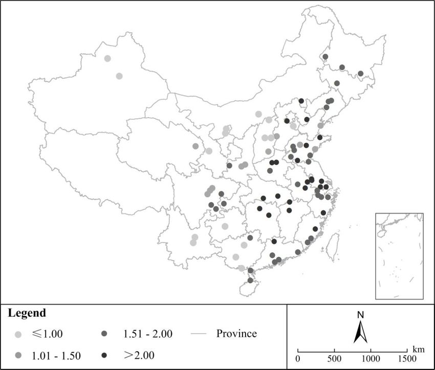
direction and non-dominant directions. Figure 1 shows the spatial distribution of this
NEIGHBOR variable. It highlights which cities are suffering the most from
surrounding smoke emissions. The top five cities that suffer most from nearby cities‘
manufacturing emissions are Yantai, Weifang, Qinhuangdao, Kaifeng and Nantong.
*** Insert Figure 1 about here ***
―Sandstorm‖ represents a unique inter-regional long-distance transported
pollutant. It is mainly composed of fine sediments originating in arid and semi-arid
regions, and transported by strong winds to about seventeen provinces in China.
Similar impacts are also detected in Korea, Japan and even the west coast of the
United States and the southern British Columbia, Canada (Chun 2000; McKendry et
al. 2001). There have been growing concerns about the health damages caused by
Asian sandstorms. Based on a case study in Beijing, Ai (2003) estimates the economic
costs of sandstorm are greater than 2.9% of Beijing‘s GDP in 2000. In our model,
9
To better measure the imported pollution from all neighbor cities, we use the smoke emission information of all
287 prefecture-level (or above) cities to construct this NEIGHBOR variable.
8SANDSTORMi is city i‘s distance to the sandstorm origin (Inner Mongolia). We use a
logarithmic specification so the sandstorm‘s impact on a city‘s air quality also
diminishes when the city is located further from the sandstorm‘s origin10.
The cities north of the Huai River and Qinling Mountains (it lies at roughly 33°
latitude) receive subsidized heating in winter months, while the southern cities are not
entitled to this centralized heating. This sector creates high emissions levels because
heating‘s main energy source is coal (Almond et al. 2009).We include NORTH, which
equals to one if the city is to the north of the heating line, in Equation (1) to test for
the role of winter heating on urban PM10 pollution. Almond et al. (2009) examine the
discontinuity in air pollution above and below the Huai River due to this winter
heating effect. To see if their finding also holds in our sample, we include
NORTH_BORDER (equals to one if the city locates above but very close to the
heating line, with its latitude below 35° and above 33°) and SOUTH_BORDER
(equals to one if the city locates below but very close to the heating line, with its
latitude above 30° and below 33°), to compare if there is significant difference
between the two coefficients. The cutoff numbers are borrowed from Almond et al.
(2009).
Air quality in Chinese cities has been improving over time. The average PM10
concentration was 0.098, 0.092, 0.088 and 0.087 mg/m3 for the years 2006, 2007,
2008 and 2009, respectively. Beijing experienced a great air quality improvement in
the three years before the 2008 Olympic Game (0.162, 0.149, 0.124 mg/m 3 for 2006,
10
Ideally we could also incorporate information on the direction and velocity of the sandstorm, which are
different for different cities. Unfortunately we do not have access to accurate information. We test the robustness
of our results by considering the relationship between the sandstorm‘s direction and the city‘s spring dominant
wind direction (measured by the angle between these two. The main findings are robust to across to these changes
(available upon request).
92007, 2008 respectively) due to factory shutdowns and short-term traffic control
policies introduced. PM10 concentrations vary significantly across cities. In 2008, the
dirtiest city (Lanzhou) had a PM10 concentration level (0.149 mg/m3) four times
higher than the cleanest city (Haikou, 0.038 mg/m3).
Table 2 reports the air pollution production regressions. We estimate this
regression using OLS. Column (1) excludes the cross-boundary externality variables
and the three geographic variables. Several results emerge. First, the city size/ambient
pollution elasticity equals roughly 0.11. Cities with larger manufacturing employment
share have higher PM10 concentrations and this effect is statistically significant.
Rainfall is good for mitigating air pollution. This equation can explain 30% of the
cross-city PM10 variation. In Column (2), our two cross-boundary pollution variables
are included. They are jointly significant at 1% level and improve the explanatory
power (R2) by 0.20. Imported pollution from neighbor cities‘ manufacturing
activities has a very significant effect (at the 1% level) on a local city‘s air pollution.
A 10% decrease of the NEIGHBOR variable reduces the PM10 concentration by 1.7%.
All else equal, a city‘s pollution level declines as its distance from the sandstorm
origin in Inner Mongolian increases. In Column (3), we augment the pollution
regression model to include NORTH, NORTH_BORDER and SOUTH_BORDER.
Their coefficients are all positive (we acknowledge that NORTH may capture other
attributes of northern cities). Northern cities adjacent to the heating line have higher
PM10 concentration than southern cities adjacent to the line and this effect is
marginally significant. This is consistent with Almond et al. (2009)‘s finding of a
pollution jump just north of the winter heating border. In Column (4) we only include
10the last five explanatory variables in the regression. This set of variables performs
well in explaining the exogenous variation in a city‘s PM10 concentration. Below, we
will use this set of variables as instrumental variables in estimating a hedonic real
estate price regression.
*** Insert Table 2 about here ***
New Estimates of the Cross-City Hedonic Home Price Hedonic
Gradient
We estimate a series of pooled cross-sectional home price regressions. The
equation is presented in equation (3).
ln HPit 0 1 ln( POPit ) 2 Ai 3 X it 4 log( PM it ) it (3)
Where HPit is home price in city i in year t. The ―average home price‖
represents the average sales price of newly-built commodity housing units.
Commodity housing sales account for the majority of the housing transactions (more
than 70%) in Chinese cities. There is no reliable price data for second-hand housing
unit sales so we rely on this new housing price measure. The average annualized
home price growth rate was 17% for this time period. In 2009, the most expensive
city is Shenzhen (14,389 RMB per square meter), and the cheapest city is Songyuan
11(1,156 RMB per square meter). 11 The large cross-city price variation is due to
productivity and amenity differentials.
The ―average home price‖ in the Yearbook is sometimes criticized for its
inaccuracy in measuring price appreciation over time, due to poor quality controls.
However, the reality is that there is no reliable quality-controlled home price index for
such a large number of cities in China. Recognizing this issue, we also report results
based on a subsample of 35 major cities, which is compiled by the Institute of Real
Estate Studies at Tsinghua University (See Zheng et al. 2010 for details of the
compiling methodology). We will use this hedonic price index as a robustness test.
In equation (3), Ai are a vector of natural amenities and human capital in city i.
The key indicator for natural amenity we use here is the temperature discomfort index
(TEMP_INDEX, see Zheng et al. (2010) for definition). We will also include the city‘s
level of human capital (EDU, measured by average years of schooling). Rauch (1993)
has demonstrated using U.S data that real estate prices are higher in more educated
cities. In one specification we report below, we will also include the city‘s average
wage. We include it in our specification to show that our major results are robust to its
inclusion. In the X vector we include the city‘s manufacturing employment share
which may affect labor demand and thus affect home price in a city.
Our Instrumental Variables strategy
Past hedonic studies such as Gyourko and Tracy (1991) use ordinary least squares
to estimate the hedonic real estate gradient reported in equation (3). Such an
11
The exchange rate is roughly 7 RMB per U.S dollar.
12estimation strategy is based on the assumption that the hedonic price equation‘s error
term is uncorrelated with the regression‘s explanatory variables. But, OLS estimates
of equation (3) may yield inconsistent results of 3 for at least two different reasons.
First, air pollution is likely to be higher in those cities experiencing an economic
boom (Zabel and Kiel 2000). Such booming cities will have more industrial
activities taking place, and at the same time, households with greater incomes (due to
the boom) will be more likely to own private vehicles. As a result of these facts, such
booming cities will feature high home prices (because local labor demand is high) and
high pollution levels. This will tend to bias the OLS estimates of PM10 towards zero.
The environmental regulation ―J-curve‖ hypothesis offers a second explanation
for why local air pollution could be correlated with unobserved determinants of local
home prices. Selden and Song (1995) argue that richer nations are more likely to
enact more stringent environmental regulation. If regulation is effective at lowering
air pollution, then air pollution will be low in those areas that have effective, wealthy
government. In this case, OLS estimates are likely to overstate the direct effect of
PM10 because it proxies in part for good governance along a variety of dimensions
(such as garbage pick-up and general ―greenness‖).
Recent work in environmental economics based on U.S data offers a credible
instrumental variables strategy. Bayer et al. (2009) instrument for a city‘s air pollution
levels using nearby ―origin‖ pollution that blows over to the ―destination‖ city. Such
emissions raise the destination‘s local ambient air pollution levels but are unlikely to
be correlated with the hedonic pricing equation‘s error term. Other studies also find
cross-border emission transport may contribute substantially to both source and
13downwind regions, therefore one city or region‘s air quality depends upon its own
emissions and is affected by emissions from surrounding cities and regions (Tong and
Mauzerall 2008; Liu et al. 2008).
We will follow this strategy to address the concern that PM10 is correlated with
the error term in equation (3). In estimating equation (3), our X vector includes the
city‘s population, manufacturing share, human capital level, and the temperature
index. In estimating our first stage instrumental variables regression (see equation (1)),
we include these X variables as explanatory variables. As in any instrumental
variables regression, in addition to the X vector, the analyst must identify a set of
variables that are correlated with the endogenous variable (PM) but should not
directly appear in the outcome equation (3). We instrument for ln(PM) using the two
cross-boundary externality variables (NEIGHBOR, SANDSTORM) and the three
geographic variables (NORTH, NORTH_BORDER, SOURTH_BORDER).
We also address the concern about the potential endogeneity of city population
size (POP). As documented in the U.S literature, the population is likely to migrate to
those cities that are highly productive and that have high amenities. The error term in
equation (3) will capture the unobserved location specific attributes and the urban
population may be correlated with this. To address this concern, we use the city‘s
population twenty years ago (year 1985) and the above exogenous variables to
instrument for current city population. The year 1985 is the earliest year for which we
have access to accurate city population statistics. In addition, the year 1985 was the
very start of China‘s market economy, therefore there had been very little
14cross-city/rural-to-urban migration before that year.
Hedonic Real Estate Regression Results
Table 3 presents the hedonic real estate pricing regression results. In all of the
regressions we cluster the standard errors by city. The first four columns are for the 85
city sample using the average home price (in logarithm) as the dependent variable.
Column (1) reports OLS estimates. We find that bigger cities have higher home prices.
The cross-sectional population elasticity is about 0.28. Manufacturing employment
has a slightly positive effect on home price. We find a very significant capitalization
effect of a city‘s climate comfortableness on home prices. As expected, home prices
are significantly higher in the cities with higher human capital (measured in average
years of schooling). 12 Holding these factors constant, we find the evidence that
ambient particulate matter (PM) is negatively correlated with home prices, but the
effect is not statistically significant.
*** Insert Table 3 about here ***
As mentioned above, the OLS regressions may yield biased coefficient estimates
of the PM effect due to possible endogeneity issues. To address this, we report IV
estimates of equation (3) using the ―externality‖ variables in equation (1) (Column (4)
in Table 2) as our first stage to instruct PM, and using POP1985 to instruct POP.
In Table 3‘s Column (2), we first exclude the three geographic variables and only use
12
We acknowledge that we have a relatively ―short‖ list of city attributes compared to the U.S quality of life
literature due to data availability constraints. For example, we are unable to find city-level crime information.
15the two cross-boundary variables to instrument for PM. The IV estimates yield more
negative and significant PM elasticity than the OLS results.13 Therefore the original
OLS estimates are downward-biased to zero14. By using POP1985 to instrument for
a city‘s population POP, we can see that the coefficients of ln(POP) become smaller.
In Column (3), we further include the three geographic variables when instrumenting
for the local pollution level. The coefficient of ln(PM) becomes more negative.
Combing with the first stage‘s regression (listed at the bottom of Table 3), it is shown
that all else equal, a 10% decrease of the imported pollution from neighbors
(NEIGHBOR) is associated with a 0.76% increase in home price15.
In Column (4), we include the city‘s wage as an extra explanatory variable. We
find that prices are higher in cities that pay higher wages. As expected, due to
potential multicollinearity between wage and other explanatory variables, we see most
of the coefficients become smaller and less significant. The inclusion of this wage
variable also shrinks the PM10 capitalization coefficient but it remains negative and
statistically significant. We view this regression to be a robustness test. The typical
U.S hedonic real estate regression is viewed as a reduced form regression and the
explanatory variables are quantities of location specific attributes rather than prices
such as the price of labor (see Blomquist et al. 1988; Gyourko and Tracy 1991). Such
studies use high quality U.S micro data to estimate separate hedonic wage regressions
13
Our instrumental variables approach exploits exogenous variation in a city‘s PM10 level (due to imports of
emissions). This approach addresses the concern that a city‘s pollution is caused by such local factors as booming
industries and a rich populace that can afford to own and drive diesel vehicles. As we discussed above, such
factors will bias the OLS estimate of PM‘s implicit price to zero.
14
We find that the coefficient of MANU in the IV regressions is larger than that in OLS. This is consistent with
the downward-biased PM coefficient in the OLS regression in which booming manufacturing activities increases
both labor demand and local air pollution simultaneously.
15
In the first stage, the coefficient of ln(NEIBHOR) is 0.103, so a 10% decrease of NEIGHBOR will cause a
1.03% decrease of ln(PM), and then 0.76% decrease of home price (1.03%×0.739=0.76%).
16to measure how non-market local public goods are capitalized into both real estate
prices and wages. In this paper, our focus is solely on the determinants of local real
estate prices.16
To test the robustness of our results to different home price measures as well as to
compare our findings with those in Zheng et al. (2010), we estimate both OLS and IV
regressions using the hedonic quality-controlled home price index (HP2) and average
home price (HP1) for the subsample of 35 cities (Column (5) to (8)). The signs of the
amenity variable coefficients are quite consistent with those estimates using the
average home price measure. ln(PM) holds a significantly negative sign in both OLS
and IV regressions, and in both cases OLS estimates are downward biased, consistent
with what we find for the whole sample. The sizes of PM10 capitalization effects are
quite similar for both price measures, with that for average sale price a little bit higher
than that for hedonic price index.17 The comparability of our results across these two
different data sources raises our confidence in the 85 city sample. For the sake of
keeping a large number of cities in our sample, we will report our results based on this
average price measure thereafter.
Evidence on the Rising Demand for Clean Air
The Chinese urban population is enjoying increased income and the average
urbanite is increasingly well educated. Such households are likely to be increasingly
16
It is important to note that we include a city‘s population in each of our hedonic price regressions. This
population variable is likely to proxy for local productivity effects as the population will move to those areas that
are more productive.
17
In our 2010 RSUE paper (Zheng et al. 2010), we included the PM measure in levels in our home price hedonic
regressions. Here we include the PM measure in logarithm. It is still significant but the t-statistic is smaller. To
further verify the consistence between the two estimate versions, we estimate the regression in Column (7) with
PM measure in levels. Its coefficient is statistically significant at 5% level (t=2.15). In this paper we keep PM in
logarithm for the sake of easily calculating elasticities.
17willing to pay more to protect their health and thus willing to pay more to avoid urban
air pollution. Another trend is that the hukou constraint on labor mobility is likely to
be further phased out in the near future.18 With a higher degree of free mobility,
people can migrate to cities with higher wage and better quality of life. This arbitrage
process will mean that local public amenities will have higher capitalized prices.
In Table 4, we test these hypotheses based on our instrumental variable estimation
strategy. The first two columns report the time trend of the clean air premium.
Since our time period is relatively short (four years), we split it into two sub-periods:
2006 to 2007 and 2008 to 2009. We can see that the absolute value of this premium
rose slightly from 0.72 to 0.75. This trend is quite similar to the results reported in
Zheng et al. (2010) using data from 35 major Chinese cities during 2003 to 2006.
After we include city wage as an additional explanatory variable, this trend still
persists. The coefficient of ln(PM) is significant and its absolute value is rising over
time (these results are available on request).
We construct a HUKOU variable to measure how restrictive the hukou constraint
in a city is (see Table 1 for definition). The direct hukou restriction on labor mobility
was phased out in the wake of transition to a market economy. A worker can work in a
city without urban local hukou. As a result, population mobility, especially rural to
18
The hukou system, put in place in the 1950s, was to register people by their hometown origin and by urban
versus rural status for the purpose of regulating migration. In the wake of transition to a market economy, the
hukou‘s regulation on population mobility was relaxed. Population mobility, especially rural to urban migration,
was substantially elevated in the 1990s when urban housing market and labor market were liberalized and private
sector employment grew rapidly with the inflow of foreign direct investment (FDI) to Chinese cities. Nevertheless,
hukou remains important for rationing access to local public services and social security benefits; residents without
local urban hukou can be denied access to public schools, public health care, public pensions and unemployment
benefits in the city. hukou regulations are being eased in many Chinese cities, but the hurdles for getting hukou in
major cities remain high and few rural migrant workers could expect to overcome them. A recent study at the
Beijing Institute of Technology estimates that, tens of millions of people living in cities without urban hukou are
denied access to these public services. (―Mismanaging China's rural exodus.‖ Financial Times, 2010-03-12,
http://www.ftchinese.com/story/001031699.)
18urban migration, increased sharply in the 1990s. Therefore, urbanites in China are
able to migrate to areas that offer higher wage and better quality of life (Zheng et al.
2009). Nevertheless, the hukou remains important for rationing access to local
public services and social security benefits. Residents without local urban hukou can
be denied access to public schools, public health care, public pensions and
unemployment benefits. In our econometric specifications, a larger value of HUKOU
means a stricter entrance restriction.
In Table 4‘s Column (3) we see that those cities with higher entrance barrier
typically have higher home prices, but the price premium for clean air is smaller
(marginally significant), which is consistent with the incidence theory that in those
cities with barriers to entry it can be the case that a city can have high amenities but
relatively low real estate prices. In Column (4) and (5) we interact ln(PM) with
HIGH_INC and MID_INC (high-income cities and middle-income cities, with
low-income cities as the default category, see Table 1 for definition) as well as
SKILLCITY (cities with higher average years of schooling) dummies, respectively. We
find that as the average resident in a city becomes richer and more educated, his
willingness-to-pay for clean air does rise. Though we only find a slightly negative
interaction term in Column (5) (perhaps due to the inaccurate city-level measure of
average years to schooling), this rising capitalization trend is quite significant in
Column (4). We also interact first-tier and second-tier city dummies (FIRST_TIER,
SECOND_TIER, with third-tier cities as the default, see Table One for definition) with
ln(PM), to find that urban households in larger cities have higher willingness to pay
for clean air.
19Conclusion
Air pollution has caused severe health damage in China (Wang and Mauzerall
2006; Ho and Nielsen 2007). The World Bank (2007a, 2009) estimates that 13% of all
urban premature deaths may be due to ambient air pollution. The overall health
damage due to air pollution is roughly 3.8% of GDP in China (World Bank 2007a,
2009). Exposure to outdoor air pollutants increases the incidence of lung cancer,
cardio respiratory diseases and possibly low birth weight (Pope et al. 2002; Dockery
et al. 1993; Almond et al. 2009).
Based on a sample of 85 Chinese cities, we have presented new evidence
concerning how real estate prices are affected by local pollution. We find that real
estate prices are lower in high polluted cities and this discount is likely to grow over
time when the average resident in a city becomes richer and more-educated. The
further relaxation of the residential mobility constraint (hukou) will also push this
capitalization growth. Given that ambient air quality has recently improved in several
of China‘s cities, this rising capitalization evidence suggests that demand for clean air
is rising in China.
We have generated these facts using an instrumental variables approach where we
have exploited an important, plausibly exogenous source of variation in local air
pollution. By collecting spatial data on the cross-boundary flows in pollution from
origin to destination, we have generated more robust hedonic estimates of the value of
avoiding air pollution. Our calculations show that on average, a 10% decrease of the
20imported pollution from neighbors is associated with a 0.76% increase in home prices.
Such capitalization effects through real estate prices are sometimes ignored in policy
incidence studies when conducting cost-benefit analysis of environmental policy
analysis, however they may dominate other household welfare changes. Our paper
provides a reliable hedonic gradient estimate for estimating the social benefits
associated with public policies intended to mitigate the challenge.
As China‘s urbanites grow richer over time, their desire for living in clean, low
risk cities will rise. Costa and Kahn (2004) argue based on U.S evidence that the
statistical value of life rises faster than per-capita income growth. If this result extends
to the case of China, then this means that public policies that help to mitigate the
cross-boundary pollution problem will have increasing value to Chinese urbanites
over time. Given that air pollution is a local public bad, such air pollution reductions
will be especially valuable in heavily populated downwind areas. We recognize that
the costs of reducing the origin pollution will be an important factor in determining
optimal policy, so air pollution control efforts should not be constrained within a city
itself but need to be coordinated in a larger region.
Our results imply that public policies that reduce cross-boundary pollution flows
will simultaneously improve public health in the destination cities and lead to higher
real estate prices. Whether real estate prices rise quickly in such improving areas
hinges on the city‘s hukou system, and whether potential migrants to the city are
aware of the amenity improvements.
References
Ai, N. (2003). Socioeconomic impact analysis of yellow-dust storms: A case study in
21Beijing, China. Unpublished Master Thesis, MIT
Almond, D., Chen Y., Greenstone, M., & Li, H. (2009). Winter heating or clean air?
Unintended impacts of China‘s Huai River policy. American Economic Review
Papers and Proceedings, 99(2), 184–190.
Andrews, S. (2008). Inconsistencies in air quality metrics: ‗Blue Sky‘ days and PM10
concentrations in Beijing. Environmental Research Letters, 3(3), 034009.
Bayer, P., Keohane, N., & Timmins, C. (2009). Migration and hedonic valuation: The
case of air quality. Journal of Environmental Economics and Management, 58(1),
1–14.
Blomquist, G., Berger, M., & Hoen, J. (1988). New estimates of quality of life in
urban areas. American Economic Review, 78(1), 89–107.
Chau, K., Wong, S. , Chan, A., & Lam, K. (2006). How do people price air quality:
empirical evidence from Hong Kong. presented at the 12th Annual Conference of the
Pacific Rim Real Estate Society, Auckland, New Zealand, 22–25.
Chay, K., & Greenstone, M. (2003). The impact of air pollution on infant mortality:
Evidence from geographic variation in pollution shocks induced by a recession. The
Quarterly Journal of Economics. 118(3), 1121–1167.
Chen, Y., Ginger, Z., Kumar, N., & Shi, G. (2011). The promise of Beijing: Evaluating
the impact of the 2008 Olympic Games on air quality. NBER Working Paper 16907.
Chun, Y. (2000). The yellow-sand phenomenon recorded in the ―Joseon
Wangjosillok‖ (in Korean). Journal of the Korean Meteorological Society, 36(2),
285–292.
Costa, D., & Kahn, M. (2004). Changes in the value of life, 1940–1980. Journal of
Risk and Uncertainty, 29(2), 159–80.
Dockery, D., Pope A., Xu, X., Spengler, J., Ware, J., Fay, M., Ferris, B., & Speizer, F.
(1993). An association between air pollution and mortality in six U.S. cities. The New
England Journal of Medicine, 329(24), 1753–1759.
Edgilis. (2009). Outdoor air pollution in Asian cities: Challenges and strategies–
Hong Kong case study. Singapore.
Gyourko, J., & Tracy, J. (1991). The structure of local public finance and the quality
of life. Journal of Political Economy, 91(4), 774–806.
Ho, M. & Nielsen C. (2007). Clearing the air: The health and economic damages of
air pollution in China, MIT Press, Cambridge, MA.
Kahn, M. (1999). The silver lining of Rust Belt manufacturing decline. Journal of
Urban Economics, 46(3), 360–376.
Liu, J., Mauzerall, D. L., & Horowitz, L.W. (2008). Source-receptor relationships
between East Asian sulfur dioxide emissions and Northern Hemisphere sulfate
22concentrations. Atmospheric Chemistry and Physics, 8(14), 3721–3733.
McKendry, I., Hacker, J., Stull, R., Sakiyama, S., Mignacca, D., & Reid, K. (2001).
Long-range transport of Asian dust to the Lower Fraser Valley, British Columbia,
Canada. Journal of Geophysical Research, 106(D16), 18361–18370.
Pope, A., Burnett, R., Thun, M., Calle, E., Krewski, D., Ito, K., & Thurston, G. (2002).
Lung cancer, cardiopulmonary mortality and long-term exposure to fine particulate air
pollution. Journal of the American Medical Association, 287(9), 1132–1141.
Rauch, J. (1993). Productivity gains from geographic concentration of human capital:
Evidence from the cities. Journal of Urban Economics, 34(3), 380–400.
Rosen, S. (2002). Markets and diversity. American Economic Review, 92(1), 1–15.
Saikawa, E., Naik, V., Horowitz, L. W., Liu, J., & Mauzerall, D. L. (2009). Present
and potential future contributions of sulfate, black and organic carbon aerosols from
China to global air quality, Premature Mortality and Radiative Forcing. Atmospheric
Environment, 43(17), 2814–2822.
Selden, T., & Song, D. (1995). Neoclassical growth, the J curve for abatement, and
the inverted U curve for pollution. Journal of Environmental Economics and
Management, 29(2), 162–168.
Simonich, S. (2009). Response to comments on ―Atmospheric particulate matter
pollution during the 2008 Beijing Olympics‖. Environmental Science & Technology,
43(14), 5314-5320.
Tang, X., Shao, M., Hu, M., Wang, Z., & Zhang, J. (2009). Comment on
―Atmospheric particulate matter pollution during the 2008 Beijing Olympics‖.
Environmental Science & Technology, 43, 7588.
Tong, D., & Mauzerall, D. (2008). Summertime state-level source-receptor
relationships between nitrogen oxide emissions and downwind surface ozone
concentrations over the continental United States. Environmental Science &
Technology, 42(21), 7976–7984.
Wang, X., & Mauzerall, D. (2006). Evaluating impacts of air pollution in China on
public health: Implications for future air pollution and energy policies. Atmospheric
Environment, 40(9), 1706–1721.
Wang, W., Primbs, T., Tao, S., & Simonich, S. M. (2009). Atmospheric particulate
matter pollution during the 2008 Beijing Olympics. Environmental Science&
Technology, 43(14), 5314–5320.
World Bank. (2007a). Cost of pollution in China. Washington, DC: World Bank.
World Bank. (2007b). World development indicators. Washington, DC: World Bank.
World Bank. (2009). Cost of pollution in China. Washington, DC: World Bank.
Yao, X., Xu, X., Sabaliauskas, K., & Fang, M. (2009). Comment on ―Atmospheric
particulate matter pollution during the 2008 Beijing Olympics‖. Environmental
23Science & Technology 43, 7589.
Zabel, J., & Kiel, K. (2000). Estimating the demand for air quality in four U.S. cities.
Land Economics, 76(2), 174–194.
Zheng, S., Fu, Y., & Liu, H. (2009). Demand for urban quality of living in China:
Evidence from cross-city land rent growth. Journal of Real Estate Finance and
Economics, 38(3), 194–213.
Zheng, S., Kahn, M., & Liu, H. (2010). Towards a system of open cities in China:
Home prices, FDI flows and air quality in 35 major cities. Regional Science and
Urban Economics, 40(1): 1–10.
24Figure 1: Distribution of NEIGHBOR (Imported Emissions) in 2007
(wind-weighted)
25Table 1: Variable Definitions and Summary Statistics
Variable Definition Year Obs. Mean Std. Dev.
HP1 Average sale price of newly-built homes 2006~2009 340 3516.7 2311.5
(RMB/m2)
HP2 Quality-controlled hedonic price of 2006~2009 140 5342.0 3037.0
newly-built homes in 35 major
cities(RMB/m2)
PM PM10 concentration in air (mg/m3) 2006~2009 340 0.092 0.026
POP Non-agricultural population size 2006~2009 340 1.743 1.978
(million)
MANU Share of manufacturing employment 2006~2009 340 0.261 0.128
EDU Average year of schooling 2007 85 8.132 0.806
NEIGHBOR Imported pollution from neighbor cities 2006~2009 340 1.562 0.684
WAGE City mean annual wage per worker 2006~2009 340 2.814 0.785
(104RMB)
POP1985 Historical non-agricultural population 1985 81 0.846 1.106
size (million) in 1985
RAIN Annual rain fall (mm) 2007 85 927.9 417.6
TEMP_INDEX Temperature discomfort index 2007 85 18.1 5.55
SANDSTORM The distance to the sandstorm origin — 85 1992.0 505.9
(km)
HUKOU 2= hukou accessibility is strictly 2007 85 0.071 0.258
constrained, 1= hukou accessibility is
constrained to some extent; 0= hukou
accessibility is not constrained
HIGH_INC Binary: 1=cities with income above the 2007 85 0.330 0.473
first tri-sectional quintile in the city
income distribution, 0=otherwise
MIDDLE_INC Binary: 1=cities with income between 2007 85 0.330 0.473
the first and second tri-sectional quintile
in the city income distribution,
0=otherwise
LOW_INC Binary: 1=cities with income below the 2007 85 0.341 0.477
second tri-sectional quintile in the city
income distribution, 0=otherwise
FIRST_TIER Binary: 1=first-tier cities (Beijing, — 85 0.047 0.213
Shanghai, Shenzhen, Guangzhou),
0=otherwise
SECOND_TIER Binary: 1=second-tier cities (provincial — 85 0.365 0.484
capital/sub-provincial cities other than
the four first-tier cities), 0=otherwise
THIRD_TIER Binary: 1=third tier cities (cities other — 85 0.588 0.495
26than the above two categories),
0=otherwise
SKILLCITY Binary: 1=city‘s average years of 2007 85 0.165 0.373
schooling equals to or is above 9,
0=otherwise
NORTH Binary: 1=northern cities with winter — 85 0.353 0.481
heating (north of Huai River),
0=otherwise
NORTH_BORDER Binary: 1=northern cities adjacent to — 85 0.106 0.310
Huai River, with its latitude below 35°.
0=otherwise
SOUTH_BORDER Binary: 1=southern cities adjacent to — 85 0.200 0.402
Huai River, with its latitude above 30°.
0=otherwise
27Table 2: PM10 Production across 85 cities
Dependent variable ln(PM)
(1) (2) (3) (4)
ln(POP) 0.108*** 0.0935*** 0.0908 ***
(7.49) (7.34) (7.15)
MANU 0.278* 0.347*** 0.307**
(1.71) (2.85) (2.43)
ln(RAIN) -0.242*** -0.157*** -0.120***
(-6.51) (-5.11) (-2.68)
ln(SANDSTORM) -0.461*** -0.418*** -0.429***
(-10.01) (-8.21) (-7.90)
ln(NEIGHBOR) 0.165*** 0.138*** 0.130***
(8.93) (6.27) (7.04)
NORTH 0.0675 0.208***
(1.49) (5.77)
NORTH_BORDER 0.154*** 0.251***
(3.13) (5.76)
SOUTH_BORDER 0.0886** 0.144***
(2.42) (3.88)
Constant -0.843*** 1.972*** 1.371*** 0.684
(-3.45) (6.34) (3.30) (1.64)
YEAR2007 -0.0535 -0.0269 -0.0315 -0.0334
(-1.35) (-0.81) (-0.94) (-0.91)
YEAR2008 -0.0904** -0.0430 -0.0511 -0.0533
(-2.26) (-1.24) (-1.47) (-1.43)
YEAR2009 -0.0717 0.00899 -0.00905 -0.0577
(-1.44) (0.22) (-0.22) (-1.58)
***
33.27 54.65***
(SANDSTORM, (SANDSTORM,
*** NEIGHBOR, NEIGHBOR,
71.55
NORTH, NORTH,
Joint F-test for IV variables (SANDSTORM
NORTH_BORDE NORTH_BORDE
, NEIGHBOR)
R, R,
SOUTH_BORDE SOUTH_BORDE
R) R)
Observations 340 340 340 340
R2 0.299 0.496 0.510 0.432
t statistics in parentheses
*
p < 0.10, ** p < 0.05, *** p < 0.01
28Table 3: Cross-City Hedonic Home Price Regressions for 85 Cities
Dependent variable ln(HP1) ln(HP1) ln(HP2)
(1) (2) (3) (4) (5) (6) (7) (8)
OLS IV IV IV OLS IV OLS IV
ln(POP) 0.283*** 0.238*** 0.249*** 0.138** 0.317*** 0.159 0.337*** 0.175*
(5.07) (3.45) (3.72) (2.41) (3.71) (1.68) (3.68) (1.93)
MANU 0.0136 0.0764 0.100 0.150 0.762 0.844 0.619 0.687
(0.04) (0.15) (0.19) (0.31) (0.94) (1.01) (0.75) (0.80)
TEMP_INDEX -0.0244*** -0.0234** -0.0222** -0.0173* -0.0112 -0.0118 -0.0209* -0.0224
(-3.60) (-2.25) (-2.12) (-1.85) (-1.02) (-0.91) (-1.81) (-1.67)
ln(EDU) 1.592** 1.841** 1.774** 0.883 1.664 2.104* 0.693 1.166
(2.61) (2.34) (2.27) (1.54) (1.59) (1.81) (0.63) (0.97)
ln(PM) -0.185 -0.677** -0.739** -0.496** -0.548** -0.701* -0.516* -0.645*
(-1.38) (-2.24) (-2.40) (-2.10) (-2.04) (-1.87) (-1.94) (-1.76)
ln(WAGE) 0.408***
(5.46)
Constant 4.438*** 2.932 2.905 4.240*** 3.037 1.987 5.509** 4.476*
(3.50) (1.62) (1.59) (3.00) (1.28) (0.78) (2.35) (1.77)
Year Fixed Effects Yes Yes Yes Yes Yes Yes Yes Yes
Observations 340 324 324 324 140 140 140 140
R2 0.563 0.401 0.384 0.616 0.500 0.360 0.482 0.346
First-stage regression underlying Column (3):
ln(PM) = 2.439 + 0.141×ln(POP85) + 0.337×MANU + 0.006×TEMP_INDEX – 0.769×ln(EDU) – 0.452×ln(SANDSTORM)
+ 0.103×ln(NEIGHBOR) + 0.094×NORTH + 0.190×NORTH_BORDER + 0.080×SOUTH_BORDER + Year dummies
Joint F test for ln(SANDSTORM), ln(NEIGHBOR), NORTH, NORTH_BORDER, SOUTH_BORDER: F=33.93***
Notes: t statistics in parentheses; standard errors clustered by city.
*
p< 0.10, **p< 0.05, ***p< 0.01
29Table 4: Cross-City Hedonic Home Price Regressions Allowing For
Differential City Effects
Dependent variable ln(HP1)
(1) (2) (3) (4) (5) (6)
Year 2006~2007 2008~2009 2006~2009 2006~2009 2006~2009 2006~2009
ln(POP) 0.263*** 0.230*** 0.229*** 0.197*** 0.255*** 0.144**
(3.93) (3.30) (4.00) (3.28) (4.11) (2.25)
MANU 0.418 -0.351 0.205 0.142 0.103 0.503
(0.84) (-0.57) (0.42) (0.27) (0.19) (1.03)
TEMP_INDEX -0.0225** -0.0218** -0.0175* -0.0206** -0.0208* -0.0158*
(-2.10) (-2.09) (-1.70) (-2.05) (-1.82) (-1.86)
ln(EDU) 1.937** 1.588** 1.088 1.150* 1.291 0.631
(2.40) (2.06) (1.54) (1.74) (1.55) (0.85)
HUKOU 2.107**
(2.11)
HUKOU × ln(PM) 0.595
(1.42)
HIGH_INC ×ln(PM) -0.200***
(-4.08)
MID_INC × ln(PM) -0.0712**
(-2.30)
SKILLCITY ×ln(PM) -0.0622
(-0.86)
FIRST_TIER × ln(PM) -0.428***
(-4.17)
SECOND_TIER × ln(PM) -0.137**
(-2.41)
ln(PM) -0.721** -0.749** -0.659** -0.480* -0.725** -0.547**
(-2.55) (-2.17) (-2.23) (-1.74) (-2.38) (-2.28)
Constant 2.520 3.582* 4.359** 4.525*** 3.902** 5.268***
(1.35) (1.98) (2.45) (2.75) (2.11) (3.63)
Year Fixed Effects Yes Yes Yes Yes Yes Yes
Observations 162 162 324 324 324 324
R2 0.387 0.313 0.465 0.566 0.394 0.540
Notes: t statistics in parentheses; standard errors clustered by city.
*
p< 0.10, **p< 0.05, ***p< 0.01
30You can also read