Recurrent Neural Filters: Learning Independent Bayesian Filtering Steps for Time Series Prediction
←
→
Page content transcription
If your browser does not render page correctly, please read the page content below
Recurrent Neural Filters: Learning Independent
                                               Bayesian Filtering Steps for Time Series Prediction

                                                              Bryan Lim                                       Stefan Zohren
                                               Oxford-Man Institute of Quantitative Finance      Oxford-Man Institute of Quantitative Finance
arXiv:1901.08096v2 [stat.ML] 23 May 2019

                                                   Department of Engineering Science                 Department of Engineering Science
                                                         University of Oxford                              University of Oxford
                                                       blim@robots.ox.ac.uk                             zohren@robots.ox.ac.uk

                                                                                   Stephen Roberts
                                                                       Oxford-Man Institute of Quantitative Finance
                                                                           Department of Engineering Science
                                                                                 University of Oxford
                                                                              sjrob@robots.ox.ac.uk

                                                                                         Abstract
                                                     Despite the recent popularity of deep generative state space models, few compar-
                                                     isons have been made between network architectures and the inference steps of the
                                                     Bayesian filtering framework – with most models simultaneously approximating
                                                     both state transition and update steps with a single recurrent neural network (RNN).
                                                     In this paper, we introduce the Recurrent Neural Filter (RNF), a novel recurrent
                                                     autoencoder architecture that learns distinct representations for each Bayesian
                                                     filtering step, captured by a series of encoders and decoders. Testing this on three
                                                     real-world time series datasets, we demonstrate that the decoupled representations
                                                     learnt not only improve the accuracy of one-step-ahead forecasts while providing
                                                     realistic uncertainty estimates, but also facilitate multistep prediction through the
                                                     separation of encoder stages.

                                           1     Introduction
                                           Bayesian filtering [5] has been extensively used within the domain of time series prediction, with
                                           numerous applications across different fields – including target tracking [18], robotics [3], finance
                                           [15], and medicine [40]. Performing inference via a series of prediction and update steps [39], Bayes
                                           filters recursively update the posterior distribution of predictions – or the belief state [43] – with
                                           the arrival of new data. For many filter models – such as the Kalman filter [23] and non-linear
                                           variants like the unscented Kalman filter [22] – deterministic functions are used at each step to adjust
                                           the sufficient statistics of the belief state, guided by generative models of the data. Each function
                                           quantifies the impact of different sources of information on latent state estimates – specifically time
                                           evolution and exogenous inputs in the prediction step, and realised observations in the update step.
                                           On top of efficient inference and uncertainty estimation, this decomposition of inference steps enables
                                           Bayes filters to be deployed in use cases beyond basic one-step-ahead prediction – with simple
                                           extensions for multistep prediction [17] and prediction in the presence of missing observations [16].
                                           With the increasing use of deep neural networks for time series prediction, applications of recurrent
                                           variational autoencoder (RVAE) architectures have been investigated for forecasting non-linear state
                                           space models [7, 27, 28, 24]. Learning dynamics directly from data, they avoid the need for explicit
                                           model specification – overcoming a key limitation in standard Bayes filters. However, these RVAEs
                                           focus predominantly on encapsulating the generative form of the state space model – implicitly

                                           Preprint. Under review.
condensing both state transition and update steps into a single representation learnt by the RVAE
decoder – and make it impossible to decouple the Bayes filter steps.
Recent works in deep generative modelling have focused on the use of neural networks to learn
independent factors of variation in static datasets – through the encouragement of disentangled
representations [32, 25] or by learning causal mechanisms [34, 42]. While a wide range of training
procedures and loss functions have been proposed [30], methods in general use dedicated network
components to learn distinct interpretable relationships – ranging from orthogonalising latent rep-
resentations in variational autoencoders [19] to learning independent modules for different causal
pathways [34]. By understanding the relationships encapsulated by each component, we can sub-
sequently decouple them for use in related tasks – allowing the learnt mechanisms to generalise to
novel domains [34, 29] or to provide building blocks for transfer learning [19].
In this paper, we introduce the Recurrent Neural Filter (RNF) – a novel recurrent autoencoder
architecture which aligns network modules (encoders and decoders) with the inference steps of the
Bayes filter – making several contributions over standard approaches. Firstly, we propose a new
training procedure to encourage independent representations within each module, by directly training
intermediate encoders with a common emission decoder. In doing so, we augment the loss function
with additional regularisation terms (see Section 5), and directly encourage each encoder to learn
functions to update the filter’s belief state given available information. Furthermore, to encourage
the decoupling of encoder stages, we randomly drop out the input dynamics and error correction
encoders during training – which can be viewed as artificially introducing missingness to the inputs
and observations respectively. Finally, we highlight performance gains for one-step-ahead predictions
through experiments on 3 real-world time series datasets, and investigate multi-step predictions
as a use case for generalising the RNF’s decoupled representations to other tasks – demonstrating
performance improvements from the recursive application of the state transition encoders alone.
2 Related Work
Given the rich literature on architectures for time series prediction and uncertainty estimation, we
focus on key works in deep generative state space modelling – with a wider survey in Appendix A.
RVAEs for State Space Modelling: The work of [7] identifies close parallels between RNNs
and latent state space models, both consisting of an internal hidden state that drives output forecasts
and observations. Using an RVAE architecture described as a variational RNN (VRNN), they build
their recognition network (encoder) with RNNs and produce samples for the stochastic hidden state
at each time point. Deep Kalman filters (DKFs) [27, 28] take this a step further by allowing for
exogenous inputs in their network and incorporating a special KL loss term to penalise state transitions
between time steps. Deep Variational Bayes Filters (DVBFs) [24] enhance the interpretability of
DKFs by modelling state transitions with parametric – e.g. linear – models, which take in stochastic
samples from the recognition model as inputs. In general, while the above models capture the
generative modelling aspects of the state space framework, their inference procedure blends both
state transition and error correction steps, obliging the recognition model to learn representations for
both simultaneously. In contrast, the RNF uses separate neural network components to directly model
the Bayes filter steps – leading to improvements in representation learning and enhanced predictive
performance in time series applications.
Hybrid Approaches: In [21], the authors take a hybrid approach with the structured variational
autoencoder (SVAE), proposing an efficient general inference framework that combines probabilistic
graphical models for the latent state with neural network observation models. This is similar in spirit
to the Kernel Kalman Filter [36], allowing for predictions to be made on complex observational
datasets – such as raw images – by encoding high dimensional outputs onto a lower dimensional
latent representation modelled with a dynamical systems model. Although SVAEs provide a degree
of interpretability to temporal dynamics, they also require a parametric model to be defined for the
latent states which may be challenging for arbitrary time series datasets. The RNF, in comparison,
can learn the relationships directly from data, without the need for explicit model specification. The
Kalman variational autoencoder (KVAE) [14] extends ideas from the SVAE, modelling latent state
using a linear Gaussian state space model (LGSSM). To allow for non-linear dynamics, the KVAE
uses a recognition model to produce time-varying parameters for the LGSSM, weighting a set of K
constant parameters using weights generated by a neural network. Deep State Space Models (DSSM)
2[37] investigate a similar approach within the context of time series prediction, using an RNN to
generate parameters of the LGSSM at each time step. While the LGSSM components do allow
for the application of the Kalman filter, we note that updates to the time-varying weights from the
RNN once again blend the prediction and update steps – making the separation of Bayes filter steps
and generalisation to other tasks non-trivial. On the other hand, the RNF naturally supports simple
extensions (e.g. multistep prediction) similarly to other Bayes filter – due to the close alignment
of the RNF architecture with the Bayes filter steps and the use of decoupled representations across
encoders and decoders.
3 Problem Definition
T
Let yt = [yt (1), . . . , yt (O)] be a vector of observations, driven by a set of stochastic hidden states
T
xt = [xt (1), . . . , xt (J)]T and exogenous inputs ut = [ut (1), . . . , ut (I)] . We consider non-linear
state space models of the following form:
yt ∼ Π f (xt ) (1)
xt ∼ N µ(xt−1 , ut ), Σ(xt−1 , ut ) (2)
where Π is an arbitrary distribution parametrised by a non-linear function f (xt ), with µ(·) and Σ(·)
being mean and covariance functions respectively.
Bayes filters allow for efficient inference through the use of a belief state, i.e. a posterior distribution
of hidden states given past observations y1:t = {y1 , . . . , yt } and inputs u1:t = {u1 , . . . , ut }. This
is achieved through the maintenance of a set sufficient statistics θt – e.g. means and covariances
θt ∈ {µt , Σt } – which compactly summarise the historical data:
p(xt |y1:t , u1:t ) = bel(xt ; θt ) (3)
= N (xt ; µt , Σt ) (4)
where bel(.) is a probability distribution function for the belief state.
For filters such as the Kalman filter – and non-linear variants like the unscented Kalman filter [22] –
θt is recursively updated through a series of prediction and update steps which take the general form:
Prediction (State Transition): θ̃t = φu (θt−1 , ut ) (5)
Update (Error Correction): θt = φy θ̃t , yt (6)
where φu (·) and φy (·) are non-linear deterministic functions. Forecasts can then be computed using
one-step ahead predictive distributions:
Z
p(yt |y1:t−1 , u1:t ) = p(yt |xt ) bel xt ; θ̃t dxt . (7)
In certain cases – e.g. with the Kalman filter – the predictive distribution can also be directly
parameterised using analytical functions g(.) for belief state statistics :
p(yt |y1:t−1 , u1:t ) = p yt | g(θ̃t ) . (8)
linear Gaussianstate space models, yt can be
When observations are continuous, such as in standard
modelled using a Normal distribution – i.e. yt ∼ N gµ (θ̃t ), gΣ (θ̃t ) .
4 Recurrent Neural Filter
Recurrent Neural Filters use a series of encoders and decoders to learn independent representations
for the Bayesian filtering steps. We investigate two RNF variants as described below, based on
Equations (7) and (8) respectively.
Variational Autoencoder Form (VRNF) Firstly, we capture the belief state of Equation (4) using
a recurrent VAE-based architecture. At run time, samples of xt are generated from the encoder –
approximating the integral of Equation (7) to compute the predictive distribution of yt .
3Figure 1: RNF Network Architecture
Standard Autoencoder Form (RNF) Much recent work has demonstrated the sensitivity of
VAE performance to the choice of prior distribution, with suboptimal priors either having an “over-
regularising" effect on the loss function during training [41, 45, 4], or leading to posterior collapse
[48]. As such, we also implement an autoregressive version of the RNF based on Equation (8) –
directly feeding encoder latent states into the common emission decoder.
A general architecture diagram for both forms is shown in Figure 1, with the main differences
encapsulated within z(s) (see Section 4.1.1).
4.1 Network Architecture
First, let st be a latent state that maps to sufficient statistics θt , which are obtained as outputs from
our recognition model. Per Equations (5) and (6), inference at run-time is controlled through the
recursive update of st , using a series of Long Short-Term Memory (LSTM) [20] encoders with
exponential linear unit (ELU) activations [8].
4.1.1 Encoder
To directly estimate the impact of exogenous inputs on the belief state, the prediction step, Equation
(5), is divided into two parts with separate LSTM units φx (·) and φu (·). We use ht to represent all
required memory components – i.e. both output vector and cell state for the standard LSTM – with
st being the output of the cell. A third LSTM cell φy (·) is then used for the update step, Equation
(6), with the full set of equations below.
Prediction: Update:
h 0 0
i
Propagation s̃t , h̃t = φx (ht−1 ) (9) Error Correction [st , ht ] = φy (h̃t , yt ) (11)
h i 0
Input Dynamics s̃t , h̃t = φu (h̃t , ut ) (10)
For the variational RNF, hidden state variable xt is modelled as multivariate Gaussian, given by:
xt ∼ N (m(s̃t ), V (s̃t )) (12) V (s̃t ) = diag(σ(s̃t ) σ(s̃t )) (14)
m(s̃t ) = Wm s̃t + bm (13) σ(s̃t ) = Softplus(Wσ s̃t + bσ ) (15)
where W(·) , b(·) are the weights/biases of each layer, and is an element-wise (Hadamard) product.
For the standard RNF, the encoder state s̃t is directly fed into the emission decoder leading to the
following forms for z̃t = z(s̃t ):
zVRNF (s̃t ) = xt , zRNF (s̃t ) = s̃t . (16)
44.1.2 Decoder
Given an encoder output z̃t , we use a multi-layer perceptron to model the emission function f (·):
f (z̃t ) = Wz2 ELU(Wz1 z̃t + bz1 ) + bz2 . (17)
This allows us to handle both continuous or binary observations using the output models below:
ytcontinuous ∼ N fµ (z̃t ) , Γ(z̃t ) , (18) ytbinary ∼ Bernoulli Sigmoid(f (z̃t )) . (19)
where Γ(z̃t ) = diag (gσ (z̃t )) is a time-dependent diagonal covariance matrix, and gσ (z̃t ) =
Softplus(fσ (z̃t )).
For ytcontinuous , the weights Wz1 , bz1 are shared between fµ (·) and fσ (·) – i.e. both observation
means and covariances are generated from the same encoder hidden layer.
4.2 Handling Missing Data and Multistep Prediction
In line with standard Bayes filters, the RNF stages can be decoupled at run-time – with different
combinations made depending on the data available at each time step.
Figure 2 demonstrates how the
RNF stages can be combined to
accommodate missing data, noting
that the colour scheme of the en-
coders/decoders shown matches that
of Figure 1. From the schematic, the
propagation encoder – which is re-
sponsible for changes to the belief
state due to time evolution – is always
applied, with the input dynamics and
error correction encoders only used
when inputs or observations are ob-
served respectively. Where inputs are
available, the emission decoder is ap-
plied to the input dynamics encoder
to generate predictions at each step. Figure 2: RNF Configuration with Missing Data
Failing that, the decoder is applied to
the propagation encoder alone.
Multistep forecasts can also be treated as predictions in the absence of inputs or observations, with
the encoders used to project the belief state in a similar fashion to missing data.
5 Training Methodology
Considering the joint probability for a trajectory of length T , we train the standard RNF by minimising
the negative log-likelihood of the observations. For continuous observations, this corresponds to the
Gaussian likelihoods from Equation (18):
T
X
LRNF (ω, s̃1:T ) = − log p(yt |s̃t ), (20)
t=1
J 2
1X yt (j) − fµ (j, s̃t )
log p(yt |s̃t ) = − log(2πgσ (j, s̃t )2 ) + , (21)
2 j=1 gσ (j, s̃t )
where ω are the weights of the deep neural network, fµ (j, z̃t ) is the j-th element of fµ (z̃t ), and
gσ (j, z̃t ) the j-th element of gσ (z̃t ).
5For the VRNF, we adopt the Stochastic Gradient Variational Bayes (SGVB) estimator of [26] for our
VAE evidence lower bound, expressing our loss function as:
T L
X 1X (i)
LVRNF (ω, s̃1:T ) = log p(yt |xt (s̃t )) − KL q(x1:T ) || p(x1:T ) , (22)
t=1
L i=1
(i)
where L is the number of samples used for calibration, xk (s̃k ) is the i-th sample given the latent
state s̃k , and KL ·) is the KL divergence term defined based on the priors in Section 5.1.
5.1 VAE Priors for VRNF
Using the generative model for xt in Equation (2), we consider the definition of two priors for the
VRNF, as described briefly below. A full definition can be found in Appendix B, which also includes
derivations for the KL term used in LVRNF (ω, s̃1:T ).
Kalman Filter Prior (VRNF-KF) Considering a linear Gaussian state space form for Equations
(1) and (2), we can apply the Kalman filtering equations to obtained distributions for xt at each time
step (e.g. p(xt |y1:t , u1:t )). This also lets us to analytically define how the means and covariances of
the belief state change with different sets of information – aligning the VRNF’s encoder stages with
the filtering equations.
Neural Network Prior (VRNF-NN) In the spirit of the DKF [27], the analytical equations from
the Kalman filter prior above can also be approximated using simple multilayer perceptrons. This
would also allow belief state updates to accommodate non-linear states space dynamics, making it a
less restrictive prior model.
5.2 Encouraging Decoupled Representations
Combined Encoder Training To learn decoupled representations for the Bayesian filtering steps,
the same emissions decoder is applied to all encoders during training as indicated in Figure 1, with
encoders trained jointly using the combined loss function below:
Additional Regularisation Terms
z }| {
0
Lcombined (ω, y1:T , u1:T ) = L(ω, s̃1:T ) + αx L(ω, s̃1:T ) + αy L(ω, s1:T ) . (23)
| {z } | {z } | {z }
Input Dynamics Propagation Error Correction
The inclusion of additional stages can also be interpreted as to regularisation terms for the standard
VRNF or RNF loss functions – weighted by constants αx and αy to controls the relative importance
of the intermediate encoder representations. For our main experiments, we place equal importance
on all encoders, i.e. αx = αy = 1, to facilitate the subsequent separation of stages for multistep
prediction – with a full ablation analysis performed to assess the impact of various α settings during
training. Furthermore, the error correction component φy (·) can also be interpreted as a pure auto-
encoding step for the latest observation, recovering distributions of yt based on filtered distributions
of xt |y1:t , u1:t . This hence obliges the network to learn representations for st that are able to
reconstruct the current observation when it is available.
Introducing Artificial Missingness Next, to encourage the clean separation of encoder stages for
generalisation to other tasks, we break dependencies between the encoders by introducing artificial
missingness into the dataset, by randomly dropping out inputs and observations with a missingness
rate r. As encoders are only applied where data is present (see Figure 2), input dynamics and error
correction encoders are hence randomly skipped over during training – encouraging the encoder
to perform regardless of which encoder stage preceded it. This also bears a resemblance to input
dropout during training, which we apply to competing RVAE benchmarks to ensure comparability.
6 Performance Evaluation
6.1 Time Series Datasets
We conduct a series of tests on 3 real-world time series datasets to evaluate performance:
6VRNF VRNF
LSTM DeepAR DSSM VRNN DKF RNF
-KF -NN
Electricity 1.000 1.028 1.131 2.264 0.981 0.973 0.964 0.882
Volatility 1.000 3.914 0.989 0.980 0.972 1.894 1.271 0.966*
Quote 1.000* 1.046 1.048 3.913 1.049 1.048 1.050 1.045
Table 1: Normalised MSEs For One-Step-Ahead Predictions
VRNF VRNF
LSTM DeepAR DSSM VRNN DKF RNF
-KF -NN
Electricity - 0.966 0.964 0.981 0.965 0.320 0.271 0.961*
Volatility - 0.997* 0.999 1.000 1.000 1.000 1.000 1.000
Quote - 0.997 0.991 0.005 0.998 0.924* 0.992 0.997
Table 2: Coverage Probability Of One-Step-Ahead 90% Prediction Interval
Input VRNF VRNF
τ= LSTM DeepAR DSSM VRNN DKF RNF
Type -KF -NN
Unknown 5 4.56 4.50 4.89 4.63 4.44 4.88 3.51 3.49*
10 7.69 7.44 7.84 7.56 7.47 11.24 6.31* 6.70
15 9.83 9.40 9.78 9.58 9.48 15.53 8.10* 9.93
20 11.14 10.65 10.96 10.81 10.75 17.85 9.28* 10.27
Known 5 1.37 4.50 4.60 4.57 1.07 1.38 1.00 0.94*
10 1.48 7.44 7.00 7.44 1.09 1.40 1.00 0.96*
15 1.56 9.40 8.74 9.42 1.10 1.40 1.00 0.97*
20 1.64 10.65 9.97 10.63 1.11 1.40 1.00 0.97*
Table 3: Normalised MSEs For Multistep Predictions On Electricity Dataset
Base No Skip αx = 0, αx = 1, αx = 0, No Skip,
αy = 1 αy = 0 αy = 0 αx = 0,
αy = 0
Metric Datasets (RNF) (RNF-NS) (RNF-NP) (RNF-NU) (RNF-IO) (RNF-NSIO)
Norm. Electricity 0.882 0.937 0.965 0.857 0.871 0.798*
MSEs Volatility 0.966 0.969 0.961* 0.971 1.001 0.979
Quote 1.045 1.049 1.075 1.047 1.069 1.041*
PICP Electricity 0.961* 0.963 0.964 0.971 0.963 0.963
Volatility 1.000 1.000 0.999* 1.000 0.999* 0.999*
Quote 0.997 0.988 1.000 0.895* 0.951 0.986
Table 4: Ablation Analysis – One-Step-Ahead Prediction Results
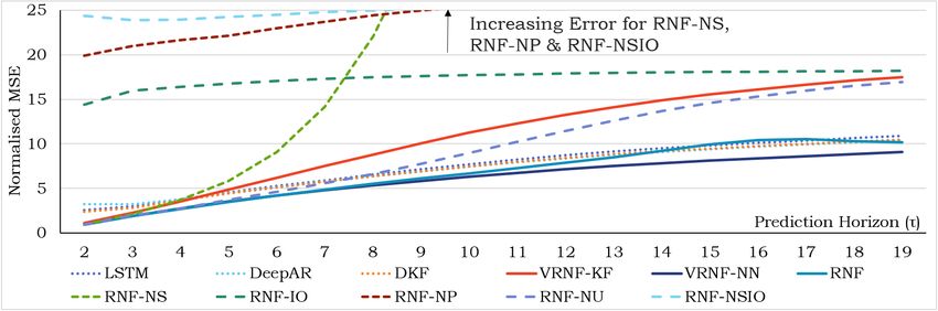
Figure 3: Ablation Analysis – Electricity Multistep MSEs For Predictions With Unknown Inputs
71. Electricity: The public UCI Individual Household Electric Power Consumption Data [10]
2. Volatility: A 30-min realised variance [1] dataset for 30 different stock indices
3. Quote: A high-frequency market microstructure dataset containing Barclays Level-1 quote
data from Thomson Reuters Tick History (TRTH)
Details on input/output features and preprocessing are fully documented in Appendix D for reference.
6.2 Conduct of Experiment
Metrics: To determine the accuracy of forecasts, we evaluate the mean-squared-error (MSE)
for single-step and multistep predictions – normalising each using the MSE of the one-step-ahead
simple LSTM forecast. As observations are 1D continuous variables for all our datasets, we evaluate
uncertainty estimates using the prediction interval coverage probability (PICP) of a 90% prediction
interval, defined as:
T
1X 1, if ψ(0.05, t) < yt < ψ(0.95, t)
PICP = ct , (24) ct = (25)
T 0, otherwise
t=1
where ψ(0.05, t) is the 5th percentile of samples from N (f (xt ), Γ). For prediction interval tests,
we omitted the pure LSTM benchmark – which is purely deterministic – from our evaluation.
Benchmarks: We compare the VRNF-KF, VRNF-NN and standard RNF against a range of RNN,
autoregressive and RVAE benchmarks – including the standard LSTM, DeepAR Model [13], Deep
State Space Model (DSSM) [37], Variational RNN (VRNN) [7], and Deep Kalman Filter (DKF) [27].
For multistep prediction, we consider two potential use cases for exogenous inputs: (i) when future
inputs are unknown beforehand and imputed using their last observed values, and (ii) when inputs
are known in advance and used as given. When models require observations of yt as inputs, we
recursively feed outputs from the network as inputs at the next time step. These tweaks allow
the benchmarks to be used for multistep prediction without modifying network architectures. For
the RNF, we consider the application of the propagation encoder alone for the former case, and a
combination of the propagation and input dynamics encoder for the latter – as detailed in Section 4.2.
Training Details: Please refer to Appendix C for full details on network calibration.
6.3 Results and Discussion
On the whole, the standard RNF demonstrates the best overall performance – improving MSEs
in general for one-step-ahead and multistep prediction, while retaining comparative PICPs with
competing benchmarks. From the one-step-ahead MSEs in Table 1, the RNF outperforms all
benchmarks in the Electricity and Volatility datasets, while coming in second only after the standard
LSTM for the Quote dataset. Focusing on the Electricity dataset for multistep predictions in Table 3,
the VRNF-NN and RNF demonstrate improvements on all benchmarks and horizons when inputs are
known. With unknown inputs, the recursive application of the propagation encoder leads to better
performance versus non-RNF benchmarks up to τ = 15, with comparable performance beyond.
As mentioned in Section 4, the challenges of prior selection for VAE-based methods can be seen from
the PICPs in Table 2 – with small PICPs for VRNN models indicative of miscalibrated distributions
in the Electricity data, and the poor MSEs and PICPs for the VRNN indicative of posterior collapse
on the Quote data. However, this can also be beneficial when applied to appropriate datasets – as
seen from the closeness of the VRNN-KF’s PICP to the expected 90% on the Quote data. As such,
the autoregressive form of standard RNF leads to more reliable performance from both a prediction
accuracy and uncertainty perspective – doing away with the need to define a prior for xt .
An ablation analysis was conducted to evaluate the effects of encoder skipping and the regulari-
sation weights during training, with results shown in Table 4 and Figure 3. While the benefits of
regularisation and skipping are largely dataset dependent – with slight improvements even observed
when they are removed (RNF-NSIO) – they play a critical role in the encouragement of decoupled
representations. This can be seen from the Multistep MSEs in Figure 3 which compares various RNF
combinations against the best performers in each benchmark category – with all variants without en-
coder skipping and full regularisation demonstration poor performance over the horizon, particularly
in cases when the propagation stage is not added to the training loss.
87 Conclusions
In this paper, we introduce a novel recurrent autoencoder architecture, which we call the Recurrent
Neural Filter (RNF), to learn decoupled representations for the Bayesian filtering steps – consisting
of separate encoders for state propagation, input and error correction dynamics, and a common
decoder to model emission. Based on experiments with three real-world time series datasets, the
direct benefits of the architecture can be seen from the improvements in one-step-ahead predictive
performance, while maintaining comparable uncertainty estimates to benchmarks. Due to its modular
structure and close alignment with Bayes filter steps, we also show the potential to generalise the
RNF to similar predictive tasks – as seen from improvements in multistep prediction using extracted
state transition encoders.
9References
[1] Torben Andersen, Tim Bollerslev, Francis Diebold, and Paul Labys. Modeling and forecasting realized
volatility. Econometrica, 71(2):579–625, 2003.
[2] Torben G. Andersen and Tim Bollerslev. Intraday periodicity and volatility persistence in financial markets.
Journal of Empirical Finance, 4(2):115 – 158, 1997.
[3] Timothy D. Barfoot. State Estimation for Robotics. Cambridge University Press, New York, NY, USA,
2017.
[4] Samuel R. Bowman, Luke Vilnis, Oriol Vinyals, Andrew M. Dai, Rafal Józefowicz, and Samy Bengio.
Generating sentences from a continuous space. CoRR, abs/1511.06349, 2015.
[5] James V. Candy. Bayesian Signal Processing: Classical, Modern and Particle Filtering Methods. Wiley-
Interscience, New York, NY, USA, 2009.
[6] Krzysztof Choromanski, Carlton Downey, and Byron Boots. Initialization matters: Orthogonal predictive
state recurrent neural networks. In International Conference on Learning Representations (ICLR 2018),
2018.
[7] Junyoung Chung, Kyle Kastner, Laurent Dinh, Kratarth Goel, Aaron C Courville, and Yoshua Bengio. A
recurrent latent variable model for sequential data. In Advances in Neural Information Processing Systems
28 (NIPS 2016). 2015.
[8] Djork-Arne Clevert, Thomas Unterthiner, and Sepp Hochreiter. Fast and accurate deep network learning by
exponential linear units (ELUs). In International Conference on Learning Representations (ICLR 2016),
2016.
[9] Zihang Dai, Zhilin Yang, Yiming Yang, Jaime G. Carbonell, Quoc V. Le, and Ruslan Salakhutdinov.
Transformer-XL: Attentive language models beyond a fixed-length context. CoRR, abs/1901.02860, 2019.
[10] Dua Dheeru and Efi Karra Taniskidou. UCI machine learning repository – individual household electric
power consumption data set, 2017.
[11] Andreas Doerr, Christian Daniel, Martin Schiegg, Nguyen-Tuong Duy, Stefan Schaal, Marc Toussaint, and
Trimpe Sebastian. Probabilistic recurrent state-space models. In Proceedings of the 35th International
Conference on Machine Learning (ICML 2018), 2018.
[12] Carlton Downey, Ahmed Hefny, Byron Boots, Geoffrey J Gordon, and Boyue Li. Predictive state recurrent
neural networks. In Advances in Neural Information Processing Systems 30 (NIPS 2017). 2017.
[13] Valentin Flunkert, David Salinas, and Jan Gasthaus. Deepar: Probabilistic forecasting with autoregressive
recurrent networks. CoRR, abs/1704.04110, 2017.
[14] Marco Fraccaro, Simon Kamronn, Ulrich Paquet, and Ole Winther. A disentangled recognition and
nonlinear dynamics model for unsupervised learning. In Advances in Neural Information Processing
Systems 30 (NIPS 2017). 2017.
[15] Himadri Ghosh, Bishal Gurung, and Prajneshu. Kalman filter-based modelling and forecasting of stochastic
volatility with threshold. Journal of Applied Statistics, 42(3):492–507, 2015.
[16] A. C. Harvey and R. G. Pierse. Estimating missing observations in economic time series. Journal of the
American Statistical Association, 79(385):125–131, 1984.
[17] Andrew Harvey. Forecasting, Structural Time Series Models and the Kalman Filter. Cambridge University
Press, 1991.
[18] Anton J Haug. Bayesian estimation and tracking: a practical guide. John Wiley & Sons, Hoboken, NJ,
2012.
[19] Irina Higgins, Loic Matthey, Arka Pal, Christopher Burgess, Xavier Glorot, Matthew Botvinick, Shakir Mo-
hamed, and Alexander Lerchner. beta-VAE: Learning basic visual concepts with a constrained variational
framework. In International Conference on Learning Representations (ICLR 2017), 2017.
[20] Sepp Hochreiter and Jürgen Schmidhuber. Long short-term memory. Neural Computation, 9(8):1735–1780,
November 1997.
[21] Matthew Johnson, David K Duvenaud, Alex Wiltschko, Ryan P Adams, and Sandeep R Datta. Composing
graphical models with neural networks for structured representations and fast inference. In Advances in
Neural Information Processing Systems 29 (NIPS 2016). 2016.
[22] Simon J. Julier and Jeffrey K. Uhlmann. New extension of the Kalman filter to nonlinear systems. volume
3068, 1997.
[23] Rudolph Emil Kalman. A new approach to linear filtering and prediction problems. Transactions of the
ASME–Journal of Basic Engineering, 82(Series D):35–45, 1960.
10[24] Maximilian Karl, Maximilian Soelch, Justin Bayer, and Patrick van der Smagt. Deep variational Bayes
filters: unsupervised learning of state space models from raw data. In International Conference on Learning
Representations (ICLR 2017), 2017.
[25] Hyunjik Kim and Andriy Mnih. Disentangling by factorising. In Proceedings of the 35th International
Conference on Machine Learning (ICML 2018), 2018.
[26] Diederik P. Kingma and Max Welling. Auto-encoding variational Bayes. In International Conference on
Learning Representations (ICLR 2014), 2014.
[27] R. G. Krishnan, U. Shalit, and D. Sontag. Deep Kalman Filters. ArXiv e-prints, 2015.
[28] Rahul G. Krishnan, Uri Shalit, and David Sontag. Structured inference networks for nonlinear state space
models. In Proceedings of the Thirty-First AAAI Conference on Artificial Intelligence (AAAI 2017), 2017.
[29] Brenden M. Lake, Tomer D. Ullman, Joshua B. Tenenbaum, and Samuel J. Gershman. Building machines
that learn and think like people. Behavioral and Brain Sciences, 40:e253, 2017.
[30] Francesco Locatello, Stefan Bauer, Mario Lucic, Sylvain Gelly, Bernhard Schölkopf, and Olivier Bachem.
Challenging common assumptions in the unsupervised learning of disentangled representations. CoRR,
abs/1811.12359, 2018.
[31] Álvaro Cartea, Ryan Donnelly, and Sebastian Jaimungal. Enhancing trading strategies with order book
signals. Applied Mathematical Finance, 25(1):1–35, 2018.
[32] Siddharth Narayanaswamy, T. Brooks Paige, Jan-Willem van de Meent, Alban Desmaison, Noah Goodman,
Pushmeet Kohli, Frank Wood, and Philip Torr. Learning disentangled representations with semi-supervised
deep generative models. In Advances in Neural Information Processing Systems 30 (NIPS 2017), pages
5925–5935. 2017.
[33] Hannes Nickisch, Arno Solin, and Alexander Grigorevskiy. State space Gaussian processes with non-
Gaussian likelihood. In Proceedings of the 35th International Conference on Machine Learning (ICML
2018), pages 3789–3798, 2018.
[34] Giambattista Parascandolo, Niki Kilbertus, Mateo Rojas-Carulla, and Bernhard Schölkopf. Learning
independent causal mechanisms. In Proceedings of the 35th International Conference on Machine
Learning (ICML 2018), 2018.
[35] Bernardo Pérez Orozco, Gabriele Abbati, and Stephen Roberts. MOrdReD: Memory-based Ordinal
Regression Deep Neural Networks for Time Series Forecasting. CoRR, arXiv:1803.09704, 2018.
[36] L. Ralaivola and F. d’Alche Buc. Time series filtering, smoothing and learning using the kernel Kalman
filter. In Proceedings. 2005 IEEE International Joint Conference on Neural Networks, volume 3, pages
1449–1454, July 2005.
[37] Syama Sundar Rangapuram, Matthias W Seeger, Jan Gasthaus, Lorenzo Stella, Yuyang Wang, and Tim
Januschowski. Deep state space models for time series forecasting. In Advances in Neural Information
Processing Systems 31 (NeurIPS 2018). 2018.
[38] S. Sarkka, A. Solin, and J. Hartikainen. Spatiotemporal learning via infinite-dimensional Bayesian filtering
and smoothing: A look at Gaussian process regression through Kalman filtering. IEEE Signal Processing
Magazine, 30(4):51–61, July 2013.
[39] Simo Sarkka. Bayesian Filtering and Smoothing. Cambridge University Press, New York, NY, USA, 2013.
[40] R. Sukkar, E. Katz, Y. Zhang, D. Raunig, and B. T. Wyman. Disease progression modeling using hidden
Markov models. In 2012 Annual International Conference of the IEEE Engineering in Medicine and
Biology Society, pages 2845–2848, Aug 2012.
[41] Hiroshi Takahashi, Tomoharu Iwata, Yuki Yamanaka, Masanori Yamada, and Satoshi Yagi. Variational
autoencoder with implicit optimal priors. CoRR, abs/1809.05284, 2018.
[42] Valentin Thomas, Emmanuel Bengio, William Fedus, Jules Pondard, Philippe Beaudoin, Hugo Larochelle,
Joelle Pineau, Doina Precup, and Yoshua Bengio. Disentangling the independently controllable factors of
variation by interacting with the world. In NIPS 2017 Workshop on Learning Disentangled Representations,
2018.
[43] Sebastian Thrun, Wolfram Burgard, and Dieter Fox. Probabilistic Robotics (Intelligent Robotics and
Autonomous Agents). The MIT Press, 2005.
[44] A. Todd, R. Hayes, P. Beling, and W. Scherer. Micro-price trading in an order-driven market. In 2014
IEEE Conference on Computational Intelligence for Financial Engineering Economics (CIFEr), pages
294–297, March 2014.
[45] Tomczak and Welling. VAE with a VampPrior. In Proceedings of the 21st Internation Conference on
Artificial Intelligence and Statistics (AISTATS), 2018.
11[46] Ryan Turner, Marc Deisenroth, and Carl Rasmussen. State-space inference and learning with Gaussian
processes. In Proceedings of the Thirteenth International Conference on Artificial Intelligence and Statistics
(AISTATS 2010), pages 868–875, 2010.
[47] Aäron van den Oord, Sander Dieleman, Heiga Zen, Karen Simonyan, Oriol Vinyals, Alex Graves, Nal
Kalchbrenner, Andrew W. Senior, and Koray Kavukcuoglu. WaveNet: A generative model for raw audio.
CoRR, abs/1609.03499, 2016.
[48] Aaron van den Oord, Oriol Vinyals, and koray kavukcuoglu. Neural discrete representation learning. In
Advances in Neural Information Processing Systems 30 (NIPS), pages 6306–6315. 2017.
[49] Ashish Vaswani, Noam Shazeer, Niki Parmar, Jakob Uszkoreit, Llion Jones, Aidan N Gomez, Ł ukasz
Kaiser, and Illia Polosukhin. Attention is all you need. In Advances in Neural Information Processing
Systems 30 (NIPS 2017). 2017.
[50] Arun Venkatraman, Nicholas Rhinehart, Wen Sun, Lerrel Pinto, Martial Hebert, Byron Boots, Kris Kitani,
and J. Bagnell. Predictive-state decoders: Encoding the future into recurrent networks. In Advances in
Neural Information Processing Systems 30 (NIPS 2017). 2017.
[51] Ruofeng Wen and Kari Torkkola Balakrishnan (Murali) Narayanaswamy. A multi-horizon quantile
recurrent forecaster. In NIPS 2017 Time Series Workshop, 2017.
[52] A. Yadav, P. Awasthi, N. Naik, and M. R. Ananthasayanam. A constant gain kalman filter approach to
track maneuvering targets. In 2013 IEEE International Conference on Control Applications (CCA), 2013.
12Appendix for Recurrent Neural Filters
A Extended Related Work
Autoregressive Architectures: An alternative approach to deep generative mod-
elling focuses Q on the autoregressive factorisation of the joint distribution of observations
(i.e. p(y1:T ) = t p(yt |y1:t )), directly generating the conditional distribution at each step. For
instance, WaveNet [47] and Transformer [49, 9] networks use dilated CNNs and attention-based
models to build predictive distributions. While successful in speech generation and language applica-
tions, these models suffer from several limitations in the context of time series prediction. Firstly, the
CNN and attention models require the pre-specification of the amount of relevant history to use in
predictions – with the size of the look-back window controlled by the length of the receptive field or
extended context – which may be difficult when the data generating process is unknown. Furthermore,
they also rely on a discretisation of the output, generating probabilities of occurrence within each
discrete interval using a softmax layer. This can create generalisation issues for time series where
outputs are unbounded. In contrast, the LSTM cells used in the RNF recognition model remove the
need to define a look-back window, and the parametric distributions used for outputs are compatible
with unbounded continuous observations.
In other works, the use of RNNs in autoregressive architectures for time series prediction have
been explored in DeepAR models [13], where LSTM networks output Gaussian mean and standard
deviation parameters of predictive distributions at each step. We include this as a benchmark in
our tests, noting the improvements observed with the RNF through its alignment with the Bayesian
filtering paradigm.
Predictive State Representations: Predictive state RNNs (PSRNN) [6, 12, 50] use an alternative
formulation of the Bayes filter, utilising a state representation that corresponds to the statistics of
the predictive distribution of future observations. Predictions are made using a two-stage regression
approach modelled by their proposed architectures. Compared to alternative approaches, PSRNNs
only produce point estimates for their forecasts – lacking the uncertainty bounds from predictive
distributions produced by the RNF.
Non-Parametric State Space Models: Gaussian Process state space models (GP-SSMs) [46, 33]
and variational approximations [11], provide an alternative non-parametric approach to forecasting
non-linear state space models – modelling hidden states and observation dynamics using GPs. While
they have similar benefits to Bayes filters (i.e. predictive uncertainties, natural multistep prediction
etc.), inference at each time step has at least an O(T ) complexity in the number of past observations –
either via sparse GP approximations or Kalman filter formulations [38]. In contrast, the RNF updates
its belief state at each time point only with the latest observations and input, making it suitable for
real-time prediction on high-frequency datasets.
RNNs for Multistep Prediction: Customised sequence-to-sequence architectures have been
explored in [35, 51] for multistep time series prediction, typically predefining the forecast horizon,
and using computationally expensive customised training procedures to improve performance. In
contrast, the RNF does not require the use of a separate training procedure for multistep predictions –
hence reducing the computational overhead – and does not require the specification of a fixed forecast
horizon.
B VRNF Priors and Derivation of KL Term
Defining a prior distribution for the VRNF starts with the specification of a model for the distribution
of hidden state xt , conditioned on the amount of available information at each encoder to achieve
alignment with the VRNF stages. Per the generative model of Equation (2), we model xt as a
multivariate normal distribution with a mean and covariance that varies with time and the information
13present at each encoder, based on the notation below:
0 0
Propagation: p(xt |y1:t−1 , u1:t−1 ) ∼ N (β̃t , ν̃t ), (26)
Input Dynamics: p(xt |y1:t−1 , u1:t ) ∼ N (β̃t , ν̃t ), (27)
Error Correction p(xt |y1:t , u1:t ) ∼ N (βt , νt ). (28)
For the various priors defined in this section, we adopt the use of diagonal covariance matrices for the
inputs, defined as :
νt = diag(γt γt ), (29)
where γt ∈ RJ is a vector of standard deviation parameters.
This approximation helps to reduce the computational complexity associated with the matrix multi-
plications using full covariance matrices, and the O(J 2 T ) memory requirements from storing full
covariances matrices for an RNN unrolled across T timesteps.
B.1 KL Divergence Term
Considering the application of the input dynamics encoder alone (i.e. αx = αy = 0), the KL
divergence between independent conditional multivariate Gaussians at each time step can be hence
expressed analytically as:
T
p(x1 ) X p(xt |xt−1 , u1:t , y1:t−1 )
KLInput q(x1:T ) || p(x1:T ) = Eq(x1:T ) log + log (30)
q(x1 |s̃1 ) t=2 q(xt |s̃t )
T X J
( )
X γ̃t (j) σ(j, s̃t )2 + (m(j, s̃t ) − β̃t (j))2 1
= log + − , (31)
t=1 j=1
σ(j, s̃t ) 2γ̃t (j)2 2
where m(j, s̃t ), σ(j, s̃t ) are j-th elements of m(s̃t ), σ(s̃t ) as defined in Equations (13) and (15)
respectively.
The KL divergence terms are defined similarly for the propagation and error correction encoders,
using the means and standard deviations defined above.
B.2 Kalman Prior (VRNF-KF)
The use Kalman filter relies on the definition of a linear Gaussian state space model, which we specify
below:
yt = Hxt + et , (32)
xt = Axt−1 + But + t , (33)
where H, A, B are constant matrices, and et ∼ N (0, R), t ∼ N (0, Q) are noise terms with
constant noise covariances R and Q.
Propagation Assuming that inputs ut is unknown at time t, predictive distributions can still be
computed for the hidden state if we have a model for ut . In the simplest case, this can be a standard
normal distribution, i.e. ut ∼ N (c, D) – where c is a constant mean vector and D a constant
covariance matrix. Under this model, predictive distributions can be computed as below:
0
β̃t = Aβt−1 + Bc
0
= Aβt−1 + c , (34)
0
ν̃t = Aνt−1 AT + BDB T + Q
0
= Aνt−1 AT + Q , (35)
0 0
with c , Q collapsing constant terms together into a single parameters.
14Input Dynamics When inputs are known, the forecasting equations take on a similar form:
β̃t = Aβt−1 + But (36)
T
ν̃t = Aνt−1 A + Q (37)
Comparing this with the forecasting equations of the propagation step, we can express also the above
0 0
as functions β̃t and ν̃t , i.e.:
0 0
β̃t = β̃t + But − c , (38)
0 0
ν̃t = ν̃t − Q + Q. (39)
Error Correction Upon receipt of a new observation, the Kalman filter computes a Kalman Gain
Kt , using it to correct the belief state as below:
βt = (I − Kt H) β̃t − Kt Hyt , (40)
νt = (I − Kt H) ν̃t , (41)
−1
where I is an identity matrix and Kt = ν̃t H T H ν̃t H T + R
B.2.1 Approximations for Efficiency
To avoid the complex memory and space requirements associated with full matrix computations, we
make the following approximations in our Kalman Filter equations.
Constant Kalman Gain Firstly, as noted in [52], Kalman gain values in stable filters usually tend
towards a steady state value after a initial transient period. We hence fix the Kalman gain at a constant
value, and collapse constant coefficients in the error correction equations to give:
0 0
βt = K β̃t − H yt , (42)
0
νt = K ν̃t , (43)
0 0
Where K = (I − KH) and H = KH.
Independent Hidden State Dimensions Next, we assume that hidden state dimensions are inde-
pendent of one another, which effectively diagonalising state related coefficients A = diag(a) and
Q = diag(q).
0 0
Diagonalising Q , K Finally, to allow us to diagonal covariance matrices throughout our equa-
0 0 0 0
tions, we also diagonalise Q = diag(q ) and K = diag(k ).
B.2.2 Prior Definition
Using the above definitions and approximations, the Kalman filter prior can hence be expressed in
vector form using the equations below:
Propagation:
0 0
β̃t = a m(st−1 ) + c , (44)
0 0
ν̃t = a V (st−1 ) a+q . (45)
Input Dynamics:
β̃t = a m(st−1 ) + But , (46)
ν̃t = a V (st−1 ) a + q. (47)
Error Correction:
0 0
βt = k m(s̃t ) − H yt , (48)
0
νt = k V (s̃t ). (49)
15All constant standard deviation are implemented as coefficients wrapped in a softmax layer (e.g.
a = softplus(φ))) to prevent the optimiser from converging on invalid negative numbers.
In addition, we note that the form input dynamics prior is not conditioned on the propagation encoder
outputs, although we could in theory express it terms of its statistics (i.e. Equations (38) and (39)).
This to avoid converging on negative values for variances, which can be obtained from the subtraction
0
of positive constant Q , although we revisit this in this form in Section B.3.
B.3 Neural Network Prior (VRNF-NN)
Despite the convenient tractable from of the Kalman filtering equations, this relies on the use of linear
state space assumptions which might not be suitable for complex datasets. As such, we also consider
the use of multilayer perceptrons (MLP(·)) to approximate the equations described in Section B.2.2,
conditioning it on the previous active encoder stage, i.e.:
Propagation:
0
β̃t = MLPβ̃0 (m(st−1 )) (50)
0
ν̃t = MLPν̃ 0 (V (st−1 )) (51)
Input Dynamics:
β̃t = MLPβ̃ (m(s̃t ), ut ) (52)
ν̃t = MLPν̃ (V (s̃t ), ut ) (53)
Error Correction:
βt = MLPβ (m(st ), yt ) (54)
νt = MLPν (V (st ), yt ) (55)
Similar to the state transition functions used in [27], this can be interpreted as using MLPs to
approximate the true Kalman filter functions for linear datasets, while also permitting the learning of
more sophisticated non-linear models. All MLPs defined here use an ELU activation function for
their hidden layer, fixing the hidden state size to be J. Furthermore, we use linear output layers for β
MLPs, while passing that of ν MLPs through a softplus activation function to maintain positivity.
C Training Procedure for RNF
Training Details During network calibration, trajectories were partitioned into segments of 50 time
steps each – which were randomly combined to form minibatches during training. Also, networks
were trained for up to a maximum of 100 epochs or convergence. For the electricity and volatility
datasets, 50 iterations of random search were performed, using the grid found in Table 5. 20 iterations
of random search were used for the quote dataset, as the significantly larger dataset led to longer
training times for a given set of hyperparameters. A list of optimal hyperparameters settings are also
detailed in Table 6 for reference.
Hyperparameter Ranges
Dropout Rate 0.0, 0.1, 0.2, 0.3, 0.4, 0.5
State Size 5, 10, 25, 50, 100, 150
Minibatch Size 256, 512, 1024
Learning Rate 0.0001, 0.001, 0.01, 0.1, 1.0
Max Gradient Norm 0.0001, 0.001, 0.01, 0.1, 1.0, 10.0
Missing Rate 0.25, 0.5, 0.75
Table 5: Random Search Grid for Hyperparameter Optimisation
16State Sizes To ensure that consistency across all models used, we constrain both the memory state
of the RNN and the latent variable modelled to have the same dimensionality – i.e. J = dim(st ) =
dim(xt ) for the RNF. The exception is the DSSM, as the full covariance matrix of the Kalman filter
would result in a prohibitive J 2 memory requirement if left unchecked. As such, we use the constraint
where both the RNN and the Kalman filter to have the same memory capacity for the DSSM – i.e.
J = dim(st ) = dim(xt ) + dim(xt )2 .
Dropout Application Across all benchmarks, dropout was applied only onto the memory state of
the RNNs (ht ) in the standard fashion and not to latent states xt . For the LSTM, DeepAR Model and
RNF, this corresponds to applying dropout masks to the outputs and internal states of the network.
For the VRNN, DKF and DSSM, we apply dropout only to the inputs of the network – in line with
[28] to maintain comparability to the encoder skipping in the VRNFs.
Artificial Missingness Encoder skipping is restricted to only the VRNFs and standard RNF, con-
trolled bt the missing rates defined above.
Sample Generation At prediction time, latent states for the VRNN, DKF and VRNFs are sampled
as per the standard VAE case – using L = 1 during training, L = 30 for our validation error and
L = 100 for at test time. Predictions from the DeepAR Model, DSSM and standard RNF, however,
were obtained directly from the mean estimates, with that of the DSSM computed analytically using
the Kalman filtering equations. While this differs slightly from the original paper [37], it also leads to
improvements in the performance DSSM by avoiding sampling errors.
D Description of Datasets
For the experiments in Section 6, we focus on the use of 3 real-world time series datasets, each
containing over a million time steps per dataset. These use-cases help us evaluate performance for
scenarios in which real-time predictions with RNNs are most beneficial – i.e. when the underlying
dynamics is highly non-linear and trajectories are long.
D.1 Summary
Electricity: The UCI Individual Household Electric Power Consumption Dataset [10] is a time
series of 7 different power consumption metrics measured at 1-min intervals for a single household
between December 2006 and November 2010 – coming to a total of 2,075,259 time steps over 4
years. In our experiments, we treated active power as the main observation of interest, taking the
remainder to be exogenous inputs into the RNNs.
Intraday Volatility: We compute 30-min realised variances [1] for a universe of 30 different
stock indices – derived using 1-min index returns subsampled from Thomson Reuters Tick History
Level 1 (TRTH L1) quote data. On the whole, the entire dataset contains 1,706,709 measurements
across all indices, with each trajectory spanning 17 years on average. Given the strong evidence for
the intraday periodicity of returns volatility [2], we also include the time-of-day as an additional
exogenous input.
High-Frequency Stock Quotes: This dataset consists of extracted features from TRTH L1 stock
quote data for Barclays (BARC.L) – specifically forecasting microprice returns [44] using volume
imbalance as an input predictor (see Appendix D.4) – comprising a total of 29,321,946 time steps
between 03 January 2017 to 29 December 2017. From [31], volume imbalance in the limit order book
is a good predictor of the direction (sign) of the next liquidity taking order, and the price changes
immediately after the arrival of a liquidity-taking order.
D.2 Electricity
Data Processing The full trajectory was segmented into 3 portions, with the earliest 60% of
measurements for training, the next 20% as a validation set, and the final 20% as an independent test
set – with results reported in Section 6. All data sets were normalised to have zero mean and unit
standard deviations, with normalising constants computed using the training set alone.
17VRNF VRNF
Electricity LSTM DeepAR DSSM VRNN DKF RNF
-KF -NN
Dropout Rate 0.1 0.2 0.3 0.3 0 0 0 0.1
State Size 50 50 25 150 10 5 100 150
Learning Rate 0.1 0.01 0.001 0.0001 0.1 0.01 0.01 0.01
Max Norm 0.001 0.001 1 10 0.001 0.0001 0.1 0.01
Minibatch Size 256 256 512 256 256 256 1024 512
Missing Rate - - - - - 0.5 0.5 0.25
RNF RNF RNF RNF RNF
-NS -NP -NU -IO -NSIO
Dropout Rate 0.2 0.3 0.2 0.1 0.1
State Size 100 150 100 150 150
Learning Rate 0.01 0.01 0.01 0.01 0.01
Max Norm 0.001 10 0.1 10 0.1
Minibatch Size 1024 512 256 1024 256
Missing Rate - 0.25 0.25 0.5 -
VRNF VRNF
Volatility LSTM DeepAR DSSM VRNN DKF RNF
-KF -NN
Dropout Rate 0.4 0.1 0.5 0.5 0.5 0 0 0.4
State Size 25 5 5 50 10 100 150 5
Learning Rate 0.01 0.01 0.001 0.001 0.0001 0.001 0.001 0.001
Max Norm 1 0.1 0.0001 0.1 10 0.0001 10 10
Minibatch Size 512 512 512 1024 1024 256 256 256
Missing Rate - - - - - 0.5 0.5 0.75
RNF RNF RNF RNF RNF
-NS -NP -NU -IO -NSIO
Dropout Rate 0.3 0.5 0.3 0.4 0.1
State Size 5 10 5 10 5
Learning Rate 0.001 0.001 0.001 0.001 0.001
Max Norm 10 0.0001 0.01 10 10
Minibatch Size 256 256 1024 512 1024
Missing Rate - 0.5 0.25 0.75 -
VRNF VRNF
Quote LSTM DeepAR DSSM VRNN DKF RNF
-KF -NN
Dropout Rate 0.2 0.4 0.2 0.5 0.1 0 0 0.2
State Size 50 5 50 5 25 25 5 10
Learning Rate 0.01 0.1 0.01 0.1 0.01 0.001 0.1 0.1
Max Norm 1 0.1 0.0001 1 10 1 0.0001 0.0001
Minibatch Size 256 2048 256 1024 512 512 1024 1024
Missing Rate - - - - - 0.5 0.5 0.25
RNF RNF RNF RNF RNF
-NS -NP -NU -IO -NSIO
Dropout Rate 0.5 0.4 0.1 0.2 0.3
State Size 50 50 150 150 25
Learning Rate 0.01 0.001 0.001 0.01 0.1
Max Norm 1 0.001 0.001 0.0001 0.0001
Minibatch Size 256 256 256 1024 256
Missing Rate - 0.75 0.5 0.25 -
Table 6: Optimal Hyperparameter Configurations
18Summary Statistics A list of summary statistics can be seen in Table 7.
Mean S.D. Min Max
Active Power* 1.11 1.12 0.08 11.12
Reactive Power 0.12 0.11 0.00 1.39
Intensity 4.73 4.70 0.20 48.40
Voltage 240.32 3.33 223.49 252.72
Sub Metering 1 1.17 6.31 0.00 82.00
Sub Metering 2 1.42 6.26 0.00 78.00
Sub Metering 3 6.04 8.27 0.00 31.00
Table 7: Summary Statistics for Electricity Dataset
D.3 Intraday Volatility
Data Processing From the 1-min index returns, realised variances were computed as:
rk = ln pk − ln pk−1
t
X
y(t, 30) = rk2 , (56)
k=t−30
where rk is the 1-min index return at time k, ln pk is the log price at k, and y(t, 30) is the 30-min
realised variance at time t.
Before computation, the data was cleaned by only considering prices during exchange hours to avoid
spurious jumps. In addition, realised variances greater than 10 times the 200-step rolling standard
deviation were removed and replaced by its previous value – so as to reduce the impact of outliers.
For the experiments in Section 6, data across all stock indices were grouped together for training and
testing – using data prior to 2014 for training, data between 2014-2016 for validation and data from
2016 to 4 July 2018 for independent testing. Min-max normalisation was applied to the datasets, with
time normalised by the maximum trading window of each exchange and realised variances by the
max and min values of the training dataset.
Stock Index Identifiers (RICs): AEX, AORD, BFX, BSESN, BVLG, BVSP, DJI, FCHI, FTMIB,
FTSE, GDAXI, GSPTSE, HSI, IBEX, IXIC, KS11, KSE, MXX, N225, NSEI, OMXC20, OMXHPI,
OMXSPI, OSEAX, RUT, SMSI, SPX, SSEC, SSMI, STOXX50E
Summary Statistics A table of summary statistics can be found in Table 8 and give an indication
of the general ranges of trajectories.
Mean S. D. Min Max
Realised Variance* 0.0007 0.0017 0.0000 0.1013
Normalised Time 0.43 0.27 0.00 0.97
Table 8: Summary Statistics for Volatility Dataset
D.4 High-Frequency Stock Quotes
Input/Output Definitions Microprice returns yt are defined as:
Va (t)pb (t) + Vb (t)pa (t)
pt =
Va (t) + Vb (t)
pt − pt−1
yt =
pt−1
Where Vb (t) and Va (t) are the bid and ask volumes at time t respectively, pb (t) and pa (t) are the
bid/ask prices, and pt the microprice.
19Volume imbalance It is then defined as:
Vb (t) − Va (t)
It =
Vb (t) + Va (t)
Data Processing From the raw Level 1 (best bid and ask prices and volumes) data from TRTH,
we isolate measurements between 08.30 to 16.00 UK time, avoiding the effects of opening and
closing auctions in our forecasts. Furthermore, microprice returns were also normalised using an
exponentially weighting moving standard deviation with a half-life of 10,000 steps. We note that
volume imbalance by definition is restricted to be It ∈ [−1, 1], and hence does not require additional
normalisation. Finally, the data was partitioned with training data from January to June, validation
data from June to September, and the remainder for independent testing.
Summary Statistics Basic statistics can be found in Table 9, and give an indication of the range of
different variables.
Mean S. D. Min Max
Normalised Returns* 0.00 0.80 -117.72 117.13
Volume Imbalance 0.02 0.48 -1.00 1.00
Table 9: Summary Statistics for Quote Dataset
20You can also read


