REPORT 4: SEVERITY OF 2019-NOVEL CORONAVIRUS (NCOV) - IMPERIAL COLLEGE LONDON
←
→
Page content transcription
If your browser does not render page correctly, please read the page content below
10 February 2020                                         Imperial College London COVID-19 Response Team

Report 4: Severity of 2019-novel coronavirus (nCoV)
Ilaria Dorigatti+, Lucy Okell+, Anne Cori, Natsuko Imai , Marc Baguelin, Sangeeta Bhatia, Adhiratha Boonyasiri,
Zulma Cucunubá, Gina Cuomo-Dannenburg, Rich FitzJohn, Han Fu, Katy Gaythorpe , Arran Hamlet, Wes Hinsley,
Nan Hong , Min Kwun, Daniel Laydon, Gemma Nedjati-Gilani, Steven Riley, Sabine van Elsland, Erik Volz, Haowei
Wang, Raymond Wang, Caroline Walters , Xiaoyue Xi, Christl Donnelly, Azra Ghani, Neil Ferguson*. With support
from other volunteers from the MRC Centre.1

WHO Collaborating Centre for Infectious Disease Modelling
MRC Centre for Global Infectious Disease Analysis
Abdul Latif Jameel Institute for Disease and Emergency Analytics (J-IDEA)
Imperial College London
*
 Correspondence: neil.ferguson@imperial.ac.uk 1See full list at end of document. +These two authors
contributed equally.

Summary
We present case fatality ratio (CFR) estimates for three strata of 2019-nCoV infections. For cases
detected in Hubei, we estimate the CFR to be 18% (95% credible interval: 11%-81%). For cases
detected in travellers outside mainland China, we obtain central estimates of the CFR in the range 1.2-
5.6% depending on the statistical methods, with substantial uncertainty around these central values.
Using estimates of underlying infection prevalence in Wuhan at the end of January derived from
testing of passengers on repatriation flights to Japan and Germany, we adjusted the estimates of CFR
from either the early epidemic in Hubei Province, or from cases reported outside mainland China, to
obtain estimates of the overall CFR in all infections (asymptomatic or symptomatic) of approximately
1% (95% confidence interval 0.5%-4%). It is important to note that the differences in these estimates
does not reflect underlying differences in disease severity between countries. CFRs seen in individual
countries will vary depending on the sensitivity of different surveillance systems to detect cases of
differing levels of severity and the clinical care offered to severely ill cases. All CFR estimates should
be viewed cautiously at the current time as the sensitivity of surveillance of both deaths and cases in
mainland China is unclear. Furthermore, all estimates rely on limited data on the typical time intervals
from symptom onset to death or recovery which influences the CFR estimates.

SUGGESTED CITATION
Ilaria Dorigatti, Lucy Okell, Anne Cori et al. Severity of 2019-novel coronavirus (nCoV). Imperial College London
(10-02-2020), doi: https://doi.org/10.25561/77154.

                  This work is licensed under a Creative Commons Attribution-NonCommercial-NoDerivatives
                  4.0 International License.

DOI: https://doi.org/10.25561/77154                                                                 Page 1 of 14
10 February 2020 Imperial College London COVID-19 Response Team
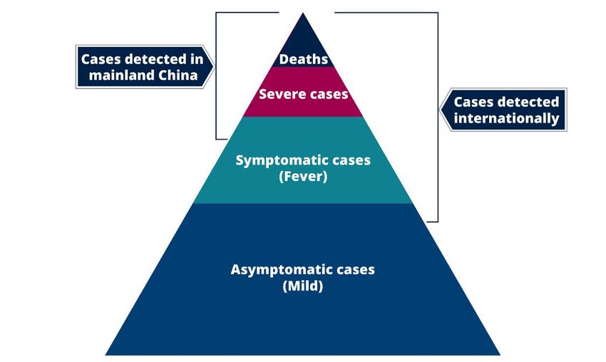
1. Introduction: Challenges in assessing the spectrum of severity
There are two main challenges in assessing the severity of clinical outcomes during an epidemic of a
newly emerging infection:
1. Surveillance is typically biased towards detecting clinically severe cases, particularly at the
start of an epidemic when diagnostic capacity is limited (Figure 1). Estimates of the proportion
of fatal cases (the case fatality ratio, CFR) may thus be biased upwards until the extent of
clinically milder disease is determined [1].
2. There can be a period of two to three weeks between a case developing symptoms,
subsequently being detected and reported and observing the final clinical outcome. During a
growing epidemic the final clinical outcome of the majority of the reported cases is typically
unknown. Dividing the cumulative reported deaths by reported cases will underestimate the
CFR among these cases early in an epidemic [1-3].
Figure 1 illustrates the first challenge. Published data from China suggest that the majority of detected
and reported cases have moderate or severe illness, with atypical pneumonia and/or acute respiratory
distress being used to define suspected cases eligible for testing. In these individuals, clinical outcomes
are likely to be more severe, and hence any estimates of the CFR are likely to be high.
Outside mainland China, countries alert to the risk of infection being imported via international travel
have instituted surveillance for 2019-nCoV infection with a broader set of clinical criteria for defining
a suspected case, typically including a combination of symptoms (e.g. cough + fever) combined with
recent travel history to the affected region (Wuhan and/or Hubei Province). Such surveillance is
therefore likely to pick up clinically milder cases as well as the more severe cases also being detected
in mainland China. However, by restricting testing to those with a travel history or link, it is also likely
to miss other symptomatic cases (and possibly hospitalised cases with atypical pneumonia) that have
occurred through local transmission or through travel to other affected areas of China.
Figure 1: Spectrum of cases for 2019-nCoV, illustrating imputed sensitivity of surveillance in
mainland China and in travellers arriving in other countries or territories from mainland China.
DOI: https://doi.org/10.25561/77154 Page 2 of 1410 February 2020 Imperial College London COVID-19 Response Team Finally, the bottom of the pyramid represents the likely largest population of those infected with either mild, non-specific symptoms or who are asymptomatic. Quantifying the extent of infection overall in the population requires random population surveys of infection prevalence. The only such data at present for 2019-nCoV are the PCR infection prevalence surveys conducted in exposed expatriates who have recently been repatriated to Japan, Germany and the USA from Wuhan city (see below). To obtain estimates of the severity of 2019-nCoV across the full severity range we examined aggregate data from Hubei Province, China (representing the top two levels – deaths and hospitalised cases – in Figure 1) and individual-level data from reports of cases outside mainland China (the top three levels and perhaps part of the fourth level in Figure 1). We also analysed data on infections in repatriated expatriates returning from Hubei Provence (representing all levels in Figure 1). 2. Current estimates of the case fatality ratio The CFR is defined as the proportion of cases of a disease who will ultimately die from the disease. For a given case definition, once all deaths and cases have been ascertained (for example at the end of an epidemic), this is simply calculated as deaths/cases. However, at the start of the epidemic this ratio underestimates the true CFR due to the time-lag between onset of symptoms and death [1-3]. We adopted several approaches to account for this time-lag and to adjust for the unknown final clinical outcome of the majority of cases reported both inside and outside China (cases reported in mainland China and those reported outside mainland China) (see Methods section below). We present the range of resulting CFR estimates in Table 1 for two parts of the case severity pyramid. Note that all estimates have high uncertainty and therefore point estimates represent a snapshot at the current time and may change as additional information becomes available. Furthermore, all data sources have inherent potential biases due to the limits in testing capacity as outlined earlier. DOI: https://doi.org/10.25561/77154 Page 3 of 14
10 February 2020                                              Imperial College London COVID-19 Response Team

  Table 1: Estimates of CFR for two severity ranges: cases reported in mainland China, and those
  reported outside. All estimates quoted to two significant figures.
Severity range         Method and data used                           Time       to      outcome         CFR
                                                                      distributions used
                       Parametric model fitted to publicly            Onset-to-death estimated           18%1
China: Epidemic        reported number of cases and deaths            from 26 deaths in China;           (95% credible
currently in           in Hubei as of 5th February, assuming          assume 5-day period from           interval: 11-81%)
Hubei                  exponential growth at rate 0.14/day.           onset to report and 1-day
                                                                      period from death to report.
                       Parametric model fitted to reported            Onset-to-death estimated           5.1%3
Outside mainland       traveller cases up to 8th February using       from 26 deaths in China;           (95% credible
China: cases in        both death and recovery outcomes               onset-to-recovery estimated        interval: 1.1%-38%)
travellers from        and inferring latest possible dates of         from 36 cases detected
mainland China         onset in traveller cases2.                     outside mainland China4.
to other               Parametric model fitted to reported            Onset-to-death estimated           5.6%1
countries or           traveller cases up to 8th February using       from 26 deaths in China.           (95% credible
territories            only death outcome and inferring                                                  interval: 2.0%-85%)
(showing a             latest possible unreported dates of
broader                onset in traveller cases2.
spectrum of            Kaplan-Meier-like non-parametric               Hazards of death and               1.2%3,4
symptoms than                                                         recovery estimated as part         (95% confidence
                       model (CASEFAT Stata module [4])
cases in Hubei,                                                       of method.                         interval: 0.9%-26%)
                       fitted to reported traveller cases up to
including milder
                       8th February using both death and
disease)
                       recovery outcomes2.
                       Scaling CFR estimate for Hubei for the         As first row                       0.9%
                       level of infection under-ascertainment                                            (95% confidence
                       estimated from infection prevalence                                               interval: 0.5%-4.0%)
                       detected in repatriation flights,
                       assuming infected individuals test
All infections         positive for 14 days
                       As previous row, but assuming                  As first row                       0.8%
                       infected individuals test positive for 7                                          (95% confidence
                       days                                                                              interval: 0.4%-3.0%)
  1Mode  quoted for Bayesian estimates, given uncertainty in the tail of the onset-to-death distribution. 2Estimates made
  without imputing onset dates in traveller cases for whom onset dates are unknown are slightly higher than when onset dates
  are imputed. 3Maximum likelihood estimate. 4This estimate relies on information from just 2 deaths reported outside
  mainland China thus far and therefore has wide uncertainty. Both of these deaths occurred a relatively short time after onset
  compared with the typical pattern in China.

  Use of data on those who have recovered among exported cases gives very similar point estimates to
  just relying on death data, but a rather narrower uncertainty range. This highlights the value of case
  follow-up data on both fatal and non-fatal cases.
  Given that the estimates of CFR across all infections rely on a single point estimate of infection
  prevalence, they should be treated cautiously. In particular, the sensitivity of the diagnostics used to
  test repatriated passengers is not known, and it is unclear when infected people might test positive,
  or how representative those passengers were of the general population of Wuhan (their infection risk
  might have been higher or lower than the general population). Additional representative studies to
  assess the extent of mildly symptomatic or asymptomatic infection are therefore urgently needed.
  Figure 2 shows projected expected numbers of deaths detected in cases detected up to 4th February
  outside mainland China over the next few weeks for different values of the CFR. If no further deaths
  are reported amongst this group (and indeed if many of those now in hospital recover and are

  DOI: https://doi.org/10.25561/77154                                                                          Page 4 of 14
10 February 2020 Imperial College London COVID-19 Response Team
discharged) in the next 5 to 10 days, then we expect the upper bound on estimates of the CFR in this
population to reduce. We note that the coming one to two weeks should allow CFR estimates to be
refined.
12
Expected number of deaths (cumulative)
10
8
6
4
2
0
21/01/2020 26/01/2020 31/01/2020 05/02/2020 10/02/2020 15/02/2020 20/02/2020
Date of death
Case Fatality Ratio
1% 3% 5%
7% 9% 11%
Observed
Figure 2: Projected numbers of deaths in cases detected outside China up to 8th February for
different values of the CFR in that population.
3. Methods
A) Intervals between onset of symptoms and outcome
During a growing epidemic, the reported cases are generally identified some time before knowing the
clinical outcome of each case. For example, during the 2003 SARS epidemic, the average time between
onset of symptoms and either death or discharge from hospital was approximately three weeks. To
interpret the relationship between reported cases and deaths, we therefore need to account for this
interval. Two factors need to be considered; a) that we have not observed the full distribution of
outcomes of the reported cases (i.e. censoring) and b) that our sample of cases is from a growing
epidemic and hence more reported cases have been infected recently compared to one to two weeks
ago. The latter effect is frequently ignored in analyses but leads to a downwards biased central
estimate of the CFR.
DOI: https://doi.org/10.25561/77154 Page 5 of 1410 February 2020 Imperial College London COVID-19 Response Team
If fOD(.) denotes the probability density function (PDF) of time from symptom onset to death, then the
PDF that we observe a death at time td with assumed onset days ago is
fOD ( )o(td − )
gOD ( | td ) = ,
f 0
OD ( ')o(td − ')d '
where o(t ) denotes the observed number of onsets that occurred at time t. For an exponentially
growing epidemic, we assume that o(t ) = o0ert where o0 is the initial number of onsets (at t=0) and
r is the epidemic growth rate. Substituting this, we get
fOD ( )e r
gOD ( | td ) =
.
f
r '
OD ( ')e d '
0
We can therefore fit the distribution g OD (.) to the observed data and correct for the epidemic growth
rate to estimate parameters for f OD (.) , the true distribution for a given estimate of r.
If we additionally assume that onsets were poorly observed prior to time Tmin then we can include
censoring:
fOD ( )e r
gOD ( | td ) = td −Tmin .
r '
fOD ( ')e d '
0
For the special case that we model f OD ( ) as a gamma distribution parameterised in terms of its
mean m and the ratio of the standard deviation to the mean, s, namely f OD ( | m, s ) , it can be shown
that
fOD ( | m / (1 + rms 2 ), s )
gOD ( | td , m ', s ') = td −Tmin ,
fOD ( ' | m / (1 + rms ), s) d '
2
0
m
where the transformed mean and standard deviation-to-mean ratios are m ' = , s ' = s.
(1 + rms 2 )
Therefore, the Bayesian posterior distribution for m and s (up to a constant factor equal to the total
probability) is proportional to the likelihood (over all intervals):
P(m, s |{ , td }) gOD ( i | td ,i , m, s)P(m, s),
i
where the product is over a dataset of observed intervals and times of death { , td } and P(m, s) is
the prior distribution for m and s. This is constant for a uniform prior distribution or can be derived,
for instance, by fitting this model to the complete dataset of observed onset-to-death intervals from
previous epidemics (e.g. in this case the 2003 SARS epidemic in Hong Kong). Note that for a fully
DOI: https://doi.org/10.25561/77154 Page 6 of 1410 February 2020 Imperial College London COVID-19 Response Team
observed epidemic, it is not necessary to account for epidemic growth provided there was no change
in clinical management (and thus the interval distribution) over time.
We can infer other interval distributions such as the onset-to-recovery distribution, f OR (.) (but also
the serial interval distribution and incubation period distribution) in a similar manner, given relevant
data on the timing of events. It should be noted that inferring all such interval distributions needs to
take account of epidemic growth.
For the analyses presented here, we fitted f OD (.) to data from 26 deaths from 2019-nCoV reported
in mainland China early in the epidemic and we fitted f OR (.) to 29 cases detected outside mainland
China. Uninformative uniform prior distributions were used for both.
The estimates of key parameters are shown in Table 2.
Table 2: Estimates of parameters for onset-to-death and onset-to-recovery distributions
Distribution Data Source mean (mode, 95% SD/mean (mode, 95%
credible interval) credible interval)
Onset-to-recovery 29 2019-CoV cases 22.2 days (18-83) 0.45 (0.35-0.62)
detected outside
mainland China
Onset-to-death 26 2019-nCoV deaths 22.3 days (18-82) 0.42 (0.33-0.6)
from mainland China
B) Estimates of the Case Fatality Ratio from individual case data
Parametric models
We can infer the CFR from individual data on dates of symptom onset, death and recovery. Continuing
our notation from above, let f OD (.) denote the distribution of times from symptom onset to death,
f OR (.) denote the distribution of times from onset to recovery, and c denote the CFR.
The probability that a patient dies on day td given onset at time to , conditional on survival to that
time is given by:
td −to +1
pd ( td − to | c, mOD , sOD ) = c f OD ( )d .
t d − to
Similarly, the probability that a patient recovers on day t r , given onset at time to ,is given by:
td −to +1
pr ( tr − to | c, mOR , sOR ) = (1 − c) f OR ( )d .
t d − to
Here mOD , sOD are the mean and standard deviation-to-mean ratio for the onset-to-death
distribution, and mOR , sOR are those for the onset-to-recovery distribution.
DOI: https://doi.org/10.25561/77154 Page 7 of 1410 February 2020 Imperial College London COVID-19 Response Team
Finally, the probability that a patient remains in hospital at the last date for which data are available,
T, is
ph (T − to | c, mOD , sOD , mOR , sOR ) = (1 − c) f OR ( )d + c f OD ( )d .
T −to T − to
The overall likelihood of all observed deaths, recoveries and cases remaining in hospital is
P(t d , t r , T | c, mOD , sOD , mOR , sOR , t o ) =
pd ( td ,i | to,i , c, mOD , sOD ) pr ( tr ,i | to ,i , c, mOR , sOR ) ph (Ti | to ,i , c, mOD , sOD , mOR , sOR )
i{dead by T } i{recovered by T } i{hospitalised at T }
It is also possible to infer c from data just on deaths and ‘non-deaths’, grouping the currently
hospitalised and recoveries together:
P(t d , t r , T | c, mOD , sOD , t o ) = pd ( td ,i | to ,i , c, mOD , sOD ) ph (T | to ,i , c, mOD , sOD , mOR , sOR )
i{dead by T } i{not dead at T }
In a Bayesian context, the posterior distribution is given by
P (c | t d , t r , t o , T )
P (t d , t r , T | c, mOD , sOD , mOR , sOR , t o ) P(mOR , sOR |{ , t d }old ) P(mOD , sOD |{ , t d }old ) P(c) dmOD dsOD dmOR dsOR
where P (mOD , sOD |{ , t d }old ) is the prior distribution for the onset-to-death distribution obtained by
fitting to previous epidemics (e.g. in this case the 2003 SARS epidemic in Hong Kong) { , t d }old , and
P(mOR , sOR |{ , t r }old ) is the comparable prior distribution for time from onset to recovery.
We assumed gamma-distributed onset-to-death and onset-to-recovery distributions (see above).
We fitted this model to the observed onset, recovery and death times in 290 international travellers
from mainland China reported up to 8th February. For approximately 50% of these travellers, the date
of onset was not reported. To allow us to fit the model to all cases, for those travellers we imputed an
estimate of the onset date as the first known contact with healthcare services – taken as the earliest
of the date of hospitalisation, date of report or date of confirmation. We note this is the latest possible
onset date and may therefore increase our estimates of CFR.
We also fitted a variant of this model where recoveries were ignored, given that they may be
systematically under-ascertained and hence introduce a bias in the estimate.
Posterior distributions were calculated numerically on a hypercube grid of the parameters to be
inferred ( c, mOD , sOD , mOR , sOR ). Marginal distributions were computed for c.
DOI: https://doi.org/10.25561/77154 Page 8 of 1410 February 2020 Imperial College London COVID-19 Response Team
Kaplan-Meier-like non-parametric model
We used a non-parametric Kaplan-Meier-like method originally developed and applied to the 2003
SARS epidemic in Hong Kong [2]. The analysis was implemented using the CASEFAT Stata Module [4].
C) Estimates of the Case Fatality Ratio from aggregated case data
With posterior estimates of f OD (.) derived from case data collected in the early epidemic in Wuhan,
it is possible to estimate the CFR from daily reports of confirmed cases and deaths in China, under the
assumption that the daily new incidence figures reported represent recent deaths and cases.
Let the incidence of deaths and onsets (newly symptomatic cases at time t be D(t ) and C (t ) ,
respectively. Given knowledge of the onset-to-death distribution, f OD (.) , the expected number of
deaths at time t is given by
D(t ) = c C (t − ) fOD ( )d
0
Assuming cases are growing exponentially as C (t ) = C0 exp(rt ) , we have
D(t ) = cC (t ) f OD ( )e − r d = czC (t )
0
where
z = f OD ( )e − r d
0
Assuming a gamma distribution form for f OD (.) , and parameterising as above in terms of the mean
and the standard deviation-to-mean ratio, m and s, respectively, one can show that z is:
1
z (r , m, s ) =
(1 + rms )
2
2 1/ s
Thus we assumed the probability of observing D(t ) deaths given C (t ) at time t is a binomial draw
from C (t ) with probability cz. The term z is a downscaling of the actual CFR, c, to reflect epidemic
growth. Heuristically, if the mean onset-to-death interval is 20 days, and the doubling time of the
epidemic is, say, 5 days, then deaths now correspond to onsets occurring when incidence of cases was
24 =16 fold smaller than today, meaning the crudely estimated CFR (cumulative deaths/ cumulative
cases) needs to be scaled up by the same factor.
Ignoring constant terms in the binomial probability not involving c, m or s , the posterior distribution
for c is:
P(c | C (t ), D(t ), m, s ) (cz (r , m, s)C (t )) D (t ) exp( −cz (r , m, s)C (t )) P(m, s) P(c)
where P(c) is the prior distribution on c (assumed uniform) and P(m, s) is the prior distribution
on the onset-to-death distribution, f OD (.) , which we took to be the posterior distribution obtained
DOI: https://doi.org/10.25561/77154 Page 9 of 1410 February 2020 Imperial College London COVID-19 Response Team by fitting to observed onset-to-death distribution for 26 cases in the early epidemic in Wuhan, itself fitted with a prior distribution based on SARS data (see above). The official case reports do not give dates of symptom onset or death, so we assumed that deaths were reported 4 days more promptly than onsets, given the delays in healthcare seeking and testing involved in confirming new cases, versus the follow-up and recording of deaths of the cases already in the database. Assuming this difference in reporting delays is longer than 4 days results in lower estimates of the CFR, while assuming the difference is shorter than 4 days gives higher estimates. Thus, we compared 45 new deaths reported on 1st February with 3156 new cases reported on 5th February. In addition, while both cases and deaths were growing approximately exponentially in the 10 days prior to 5th February, the numbers of cases have been growing faster than deaths. We assumed this reflects improved surveillance of milder cases over time, and thus used an estimate of the growth rate in deaths of r = 0.14 / day , corresponding to a 5-day doubling time. Assuming a higher value of r gives a higher estimate of the CFR. Resulting estimates of the CFR showed little variation if calculated for each of the 7 days prior to 5th February. D) Translating prevalence to incidence and estimating a CFR for all infections Translating the severity estimates in DOI: https://doi.org/10.25561/77154 Page 10 of 14
10 February 2020 Imperial College London COVID-19 Response Team
Table 1 into estimates of CFR for all cases of infection with 2019-nCoV requires knowledge of the
proportion of all infections being detected in either China or overseas. To do so we use a single point
estimate of prevalence of infection from the testing of all passengers returning on four repatriation
flights to Japan and Germany in the period 29th January – 1st February. Infection was detected in
passengers from each flight. In total 10 infections were confirmed in approximately 750 passengers
(passenger numbers are known for 3 flights and were estimated to be ~200 for the fourth). This gives
an estimate of detectable infection prevalence of 1.3% (exact 95% binomial confidence interval: 0.7%-
2.4%).
Let us assume infected individuals test positive by PCR to 2019-nCoV infection from l days before onset
of clinical symptoms to n-l days after. Then the infection prevalence at time t, y(t) is related to the
incidence of new cases, C(t) by:
n −l
y (t ) = C (t − )d / N
−l
Here N is the population of the area sampled (here assumed to be Wuhan). Assuming incidence is
growing as C (t ) = C0 exp(rt ) , with r=0.14/day (5-day doubling time), this gives
y(t ) = C (t + l ) 1 − exp(−rn) / N
Here we assume l=1 day and examine n=7 and 14 days.
Thus we estimated a daily incidence estimate of 220 (95% confidence interval: 120-400) case onsets
per day per 100,000 of population in Wuhan on 31st January assuming infections are detectable for 14
days, and 300 (95% confidence interval: 160-550) case onsets per day per 100,000 assuming infections
are detectable for 7 days. Taking the 11 million population of Wuhan city, this implied a total of 24,000
(95% confidence interval: 13,000-44,000) case onsets in the city on that date assuming infections are
detectable for 14 days, and 33,000 (95% confidence interval: 18,000-60,000) assuming infections are
detectable for 7 days. It should be noted that a number of the detected infections on the repatriation
flights were asymptomatic (at least at the time of testing), therefore these total estimates of incidence
might include a proportion of very mildly symptomatic or asymptomatic cases.
Assuming an average 4 days1 between the onset of symptoms and case report in Wuhan City, the
above estimates can be compared with the 1242 reported confirmed cases on 3rd February in Wuhan
City [5]. This implies 19-fold (95% confidence interval: 11-35) under-ascertainment of infections in
Wuhan assuming infections are detectable for 14 days (including from 1 day prior to symptoms), and
26-fold (95% confidence interval: 15-48) assuming infections are detectable for 7 days (including 1 day
prior to symptoms).
Under the assumption that all 2019-nCoV deaths are being reported in Wuhan city, we can then divide
our estimates of CFR in China by these under-ascertainment factors. Taking our 18% CFR among cases
in Hubei (first row of Table 1), this implies a CFR among all infections of 0.9% (95% confidence interval:
0.5%-4.3%) assuming infections are detectable via PCR for 14 days, and 0.8% (95% confidence interval:
0.4%-3.1%) assuming infections are detectable for 7 days.
1
This value is plausible from publicly available case reports. Longer durations between onset of symptoms and
report will lead to higher estimates of the degree of under-ascertainment.
DOI: https://doi.org/10.25561/77154 Page 11 of 1410 February 2020 Imperial College London COVID-19 Response Team
Similar estimates are obtained if one uses estimates of CFR in exported cases as the comparator: we
estimate that surveillance outside mainland China is approximately 4 to 5-fold more sensitive at
detecting cases than that in China.
E) Forward Projections of Expected Deaths in Travellers
Using our previous notation, let otravellers (t ) denote the onsets in travellers from mainland China at time
t Tmax where Tmax is the most recent time (8th February in this analysis). Using our central estimate
of the onset-to-death interval obtained from the 26 deaths in mainland China, f OD ( m, s, t ) , we obtain
an estimate of the expected number of deaths occurring at time t, D(t ) from:
D(t ) = c otravellers (t − ) f OD ( )d
0
where c is the CFR.
4. Data Sources
A) Data on early deaths from mainland China
Data on the characteristics of 39 cases who died from 2019-nCoV infection in Hubei Province were
collated from several websites. Of these, the date of onset of symptoms was not available for 5 cases.
We restricted our analysis to those who died up to 21st January leaving 26 deaths for analysis. These
data are available from website as hubei_early_deaths_2020_07_02.csv
B) Data on cases in international travellers
We collated data on 290 cases in international travellers from websites and media reports up to 8th
February. These data are available from website as international_cases_2020_08_02.csv
C) Data on infection in repatriated international Wuhan residents
Data on infection prevalence in repatriated expatriates returning to their home countries were
obtained from media reports. These data are summarised in Table 3. Further data from a flight
returning to Malaysia reported two positive cases on 5th February – giving a prevalence at this time
point of 2% which remains consistent with our estimate.
Table 3: Data on confirmed infections in passengers on repatriation flights from Wuhan.
Country of Number of Number Number Number
Destination Passengers Confirmed Confirmed Confirmed
who were who were
Symptomatic Asymptomatic
1 Japan 206 4 2 2
2 Japan 210 2 0 2
3 Japan Not reported – 2 1 1
assume 200
4 Germany 124 2 - -
5* Malaysia 207 2 0 2
DOI: https://doi.org/10.25561/77154 Page 12 of 1410 February 2020 Imperial College London COVID-19 Response Team *Not used in our analysis but noted here for completeness. 5. Acknowledgements We are grateful to the following hackathon participants from the MRC Centre for Global Infectious Disease Analysis for their support in extracting data: Kylie Ainsile, Lorenzo Cattarino, Giovanni Charles, Georgina Charnley, Paula Christen, Victoria Cox, Zulma Cucunubá, Joshua D'Aeth, Tamsin Dewé, Amy Dighe, Lorna Dunning, Oliver Eales, Keith Fraser, Katy Gaythorpe, Lily Geidelberg, Will Green, David Jørgensen, Mara Kont, Alice Ledda, Alessandra Lochen, Tara Mangal, Ruth McCabe, Kate Mitchell, Andria Mousa, Rebecca Nash, Daniela Olivera, Saskia Ricks, Nora Schmit, Ellie Sherrard- Smith, Janetta Skarp, Isaac Stopard, Hayley Thompson, Juliette Unwin, Juan Vesga, Caroline Walters. DOI: https://doi.org/10.25561/77154 Page 13 of 14
10 February 2020                                   Imperial College London COVID-19 Response Team

6. References
1.      Garske, T., et al., Assessing the severity of the novel influenza A/H1N1 pandemic. BMJ, 2009.
        339: p. b2840.
2.      Ghani, A.C., et al., Methods for estimating the case fatality ratio for a novel, emerging
        infectious disease. Am J Epidemiol, 2005. 162(5): p. 479-86.
3.      Lipsitch, M., et al., Potential Biases in Estimating Absolute and Relative Case-Fatality Risks
        during Outbreaks. PLoS Negl Trop Dis, 2015. 9(7): p. e0003846.
4.      Griffin, J. and A. Ghani, CASEFAT: Stata module for estimating the case fatality ratio of a new
        infectious disease. Statistical Software Components, 2005. S454601.
5.      People's Republic of China. National Health Commission of the People's Republic of China.
        2020 Accessed 03/02/2020]; Available from: www.nhc.gov.cn/.

DOI: https://doi.org/10.25561/77154                                                      Page 14 of 14
You can also read