(SCC) Development of a New Zealand Seafloor Community Classification - Prepared for Department of Conservation (DOC) May 2021
←
→
Page content transcription
If your browser does not render page correctly, please read the page content below
Development of a New Zealand
Seafloor Community Classification
            (SCC)
    Prepared for Department of Conservation (DOC)

                     May 2021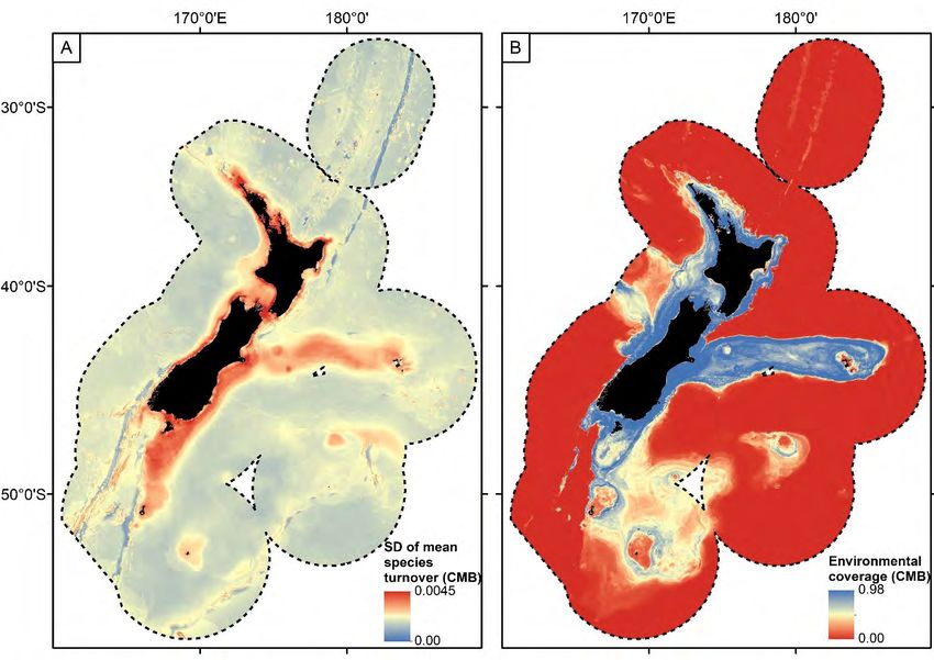
Prepared by:
Fabrice Stephenson, Ashley Rowden, Tom Brough, John Leathwick, Richard Bulmer, Dana Clark,
Carolyn Lundquist, Barry Greenfield, David Bowden, Ian Tuck, Kate Neill, Kevin Mackay, Matt
Pinkerton, Owen Anderson, Richard Gorman, Sadie Mills, Stephanie Watson, Wendy Nelson, Judi
Hewitt
For any information regarding this report please contact:
Quantitative Marine Ecologist
Benthic Marine Ecology
+64-7-859 1881
fabrice.stephenson@niwa.co.nz
National Institute of Water & Atmospheric Research Ltd
PO Box 11115
Hamilton 3251
Phone +64 7 856 7026
NIWA CLIENT REPORT No: 2020243WN
Report date: May 2021
NIWA Project: DOC19208
Quality Assurance Statement
Reviewed by: Drew Lohrer
Formatting checked by: Alex Quigley
Approved for release by: Alison MacDiarmid
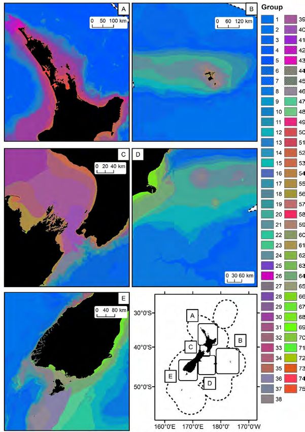
Image caption: Geographic distribution of the Seafloor Community Classification (75 groups)
© All rights reserved. This publication may not be reproduced or copied in any form without the permission of
the copyright owner(s). Such permission is only to be given in accordance with the terms of the client’s contract
with NIWA. This copyright extends to all forms of copying and any storage of material in any kind of
information retrieval system.
Whilst NIWA has used all reasonable endeavours to ensure that the information contained in this document is
accurate, NIWA does not give any express or implied warranty as to the completeness of the information
contained herein, or that it will be suitable for any purpose(s) other than those specifically contemplated
during the Project or agreed by NIWA and the Client.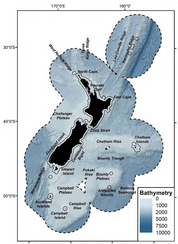
Contents
Executive summary ............................................................................................................. 6

1       Introduction .............................................................................................................. 8
        1.1      Background ............................................................................................................... 8
        1.2      Gradient Forest environmental classifications ......................................................... 8
        1.3      Aims and objectives .................................................................................................. 9

2       Biological and environmental datasets (objective 2) ................................................. 11
        2.1      Study area ............................................................................................................... 11
        2.2      Biological samples ................................................................................................... 12
        2.3      Environmental variables ......................................................................................... 16

3       Development of a Gradient Forest environmental classification (Objective 3)............ 24
        3.1      Methods .................................................................................................................. 24
        3.2      Results ..................................................................................................................... 29

Assessment of classification strength ................................................................................. 36

The New Zealand Seafloor Community Classification .......................................................... 37

4       Discussion ............................................................................................................... 43
        4.1      Critical appraisal of the Seafloor Community Classification ................................... 43
        4.2      Considerations for using the Seafloor Community Classification in spatial planning
                 ................................................................................................................................ 46
        4.3      Conclusion............................................................................................................... 48

5       Acknowledgements ................................................................................................. 49

6       Supplementary Materials 1 – Filepaths and metadata ............................................... 50
        6.1      Biological data......................................................................................................... 50
        6.2      Environmental data ................................................................................................ 52
        6.3      Model outputs ........................................................................................................ 54
        6.4      Seafloor Community Classification, example group description ............................ 55

7       Supplementary Materials 2 – Maps of biological samples.......................................... 60

8       Supplementary Materials 3 – Estuarine benthic invertebrates ................................... 64
        8.1      Data and methods .................................................................................................. 64
        8.2      Results and discussion ............................................................................................ 65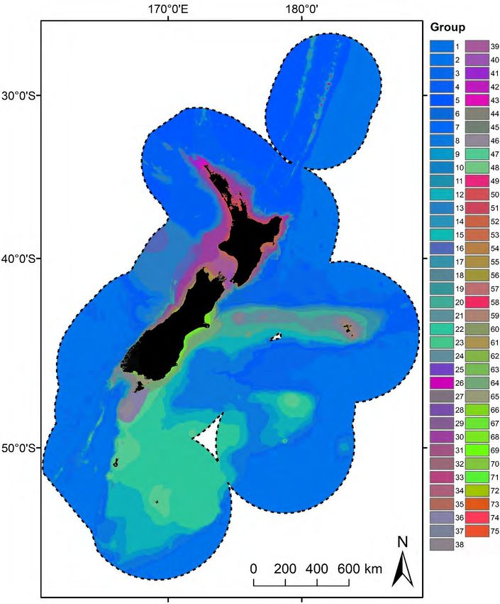
9     Supplementary Materials 4 – Compositional turnover for individual biotic groups ..... 71
      9.1     Demersal fish .......................................................................................................... 71
      9.2     Benthic invertebrates ............................................................................................. 74
      9.3     Rocky reef fish......................................................................................................... 77
      9.4     Macroalgae ............................................................................................................. 80

10    References............................................................................................................... 83

Tables
Table 2-1:      Summary of information for collated taxa records (after grooming).             12
Table 2-2:      Categories used to reflect catchability of sampling gear types.                13
Table 2-3:      Gear type codes used to reflect catchability, number of benthic invertebrate
                genera > 10 occurrence, number of unique genera > 10 occurrence and
                number of unique sample locations (see text and Table 2-2 for Gear type code
                explanations).                                                                 15
Table 2-4:      Spatial environmental predictor variables used for the Gradient Forest
                analyses.                                                                      18
                                                                   2
Table 3-1:      Mean (±SD) model fit metrics of individual taxa (R f) from bootstrapped GF
                models.                                                                        29
                                                        2
Table 3-2:      Mean (±SD) cumulative importance (R ) of environmental variables for
                bootstrapped GF models of each biotic group and for the ‘combined’
                bootstrapped GF model.                                                         30
Table 3-3: Results of the pair-wise ANOSIM analysis for the four biological datasets at varying
                levels of classification detail.                                               36
Table 6-1:      Filepaths and description of biological data.                                  50
Table 6-2:      Filepaths and description of environmental data.                               52
Table 6-3:      Filepaths and description of GF model outputs.                                 54

Figures
Figure 2-1:        Map of the study region.                                                     11
Figure 3-1:        Summary of data inputs, analyses undertaken and key outputs and
                   terminology used.                                                            27
Figure 3-2:        Mean functions fitted by bootstrapped GF models of demersal fish (blue),
                   benthic invertebrates combined across gear types (yellow), reef fish (orange),
                   macroalgae (green) samples and combined estimates (black) (R2).              32
Figure 3-3:        Mean (± SD) functions fitted by bootstrapped combined GF models of samples
                   from all biotic groups (R2).                                                 33
Figure 3-4:        Mean predicted compositional turnover in geographic and PCA space derived
                   from ‘combined’ bootstrapped Gradient Forest model fitted using samples
                   from all biotic groups.                                                      34
Figure 3-5:        Spatially explicit measures of uncertainty for compositional turnover from the
                   ‘combined’ bootstrapped Gradient Forest model fitted using samples from all
                   biotic groups                                                                35
Figure 3-6:    Dendrogram describing similarities among the seafloor community
               classification groups (75 groups) across the New Zealand marine environment.
                                                                                            38
Figure 3-7:    Principle Component Analysis (PCA) of the seafloor community classification
               groups (75 groups) for the New Zealand marine environment.                   39
Figure 3-8:    Geographic distribution of the Seafloor Community Classification (75 groups)
               derived from ‘combined’ bootstrapped Gradient Forest model.                  41
Figure 3-9:    Closeup views of parts of the geographic distribution of the Seafloor
               Community Classification (75 groups) derived from ‘combined’ bootstrapped
               Gradient Forest model.                                                       42
Figure 7-1:    Map of study region with unique locations of demersal fish used in GF analysis.
                                                                                            60
Figure 7-2:    Map of study region with unique locations of benthic invertebrates (by
               sampling gear type) used in GF analysis.                                     61
Figure 7-3:    Map of study region with unique locations of macroalgae used in GF analysis.
                                                                                            62
Figure 7-4:    Map of study region with unique locations of reef fish used in GF analysis. 63
Figure 9-1:    Mean (± SD) functions fitted by bootstrapped GF models using demersal fish
               samples (R2).                                                                71
Figure 9-2:    Mean predicted compositional turnover in geographic and PCA space derived
               from bootstrapped Gradient Forest model fitted with demersal fish samples. 72
Figure 9-3:    Spatially explicit measures of uncertainty for compositional turnover modelled
               using bootstrapped Gradient Forest model fitted with demersal fish samples.
                                                                                            73
Figure 9-4:    Mean (± SD) functions fitted by bootstrapped GF models using benthic
               invertebrate samples form combined gear types (R2).                          74
Figure 9-5:    Mean predicted compositional turnover in geographic and PCA space derived
               from bootstrapped, combined, Gradient Forest model fitted with benthic
               invertebrate samples.                                                        75
Figure 9-6:    Spatially explicit measures of uncertainty for compositional turnover modelled
               using bootstrapped Gradient Forest model fitted with benthic invertebrate
               samples.                                                                     76
Figure 9-7:    Mean (± SD) functions fitted by bootstrapped GF models using reef fish
               samples (R2).                                                                77
Figure 9-8:    Mean predicted compositional turnover in geographic and PCA space derived
               from bootstrapped Gradient Forest model fitted using reef fish samples.      78
Figure 9-9:    Spatially explicit measures of uncertainty for compositional turnover modelled
               using bootstrapped Gradient Forest model fitted with reef fish samples.      79
Figure 9-10:   Mean (± SD) functions fitted by bootstrapped GF models using macroalgae
               samples (R2).                                                                80
Figure 9-11:   Mean predicted compositional turnover in geographic and PCA space derived
               from bootstrapped Gradient Forest model fitted using macroalgae samples. 81
Figure 9-12:   Spatially explicit measures of uncertainty for compositional turnover modelled
               using bootstrapped Gradient Forest model fitted using macroalgae samples. 82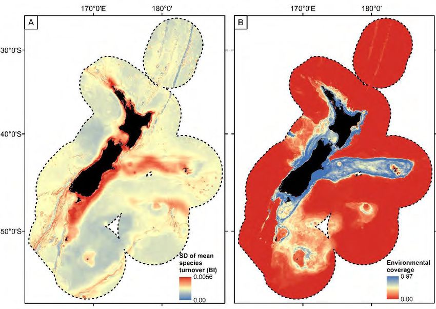
Executive summary
Marine habitats and ecosystems are under increasing pressure from human activities including
sedimentation, eutrophication, fishing, mineral extraction, waste disposal, and dredging. Well-
designed networks of marine protected areas (MPAs) can be highly effective tools for conserving
biodiversity and associated ecosystem functions and services. In New Zealand, ongoing work to
improve scientific inputs to be considered in decision-making associated with the establishment of
MPAs is supported by a MPA research programme funded via the Department of Conservation’s
(DOC’s) Biodiversity 2018 Programme. DOC commissioned the development of a fit-for-purpose,
numerical classification of the marine environment, to support ongoing MPA planning and reporting
at a national scale and complement work to develop Key Ecological Areas mapping for New Zealand.

Working with experts and members of the Marine Protected Areas Science Advisory Group (MSAG)
at a workshop held on the 9th August 2019 it was agreed that Gradient Forest (GF) models would be
used to produce a numerical classification of the seafloor environment and communities within the
New Zealand Territorial Sea and Exclusive Economic Zone (jointly referred to as the New Zealand
marine environment). Occurrence records for four biotic groups, demersal fish (317 species at 28,599
unique sample locations), benthic invertebrates (958 genera at 33,187 unique locations), macroalgae
(349 species at 3,320 unique locations) and reef fish (92 species at 339 unique locations), were used
to inform the transformation of 33 gridded environmental variables to represent spatial patterns of
taxa compositional turnover. Environmental variables were available at two resolutions: 250 m grid
resolution from the coastline to the edge of the Territorial Sea (12 NM from shore) and a 1 km grid
resolution from the edge of the Territorial Sea to the edge of the Exclusive Economic Zone.

Predicted spatial patterns of compositional turnover for taxa in each of the four biotic groups were
then combined to represent overall compositional turnover in seafloor communities, with the
combined predictors classified using a hierarchical procedure to define groups at different levels of
classification detail, (i.e., 30, 50, 75 and 100 groups). Associated uncertainty estimates of
compositional turnover for each of the seafloor communities were also produced, and an added
measure of uncertainty – coverage of the environmental space – was developed to further highlight
geographic areas where predictions may be less certain due to low sampling. A 75-group
classification – termed the New Zealand ‘Seafloor Community Classification’ (SCC) – was described.

As would be expected, the geographic and environmental patterns of the SCC closely reflect the
patterns of compositional turnover on which the SCC was based. At broad scales, SCC groups were
differentiated primarily according to oceanographic conditions such as depth and bottom
temperature. Environmental differences among groups in deep water were relatively muted, but
greater environmental differences were evident among groups at intermediate depths, particularly
with respect to bottom temperature, bottom oxygen concentration and bottom salinity. These more
pronounced environmental differences among groups at intermediate depths were aligned with
well-defined oceanographic patterns observed in New Zealand’s oceans, with a clear latitudinal
separation along the boundaries of the Subtropical Front. Environmental differences became even
more pronounced at shallow depths, where variation in more localised environmental conditions
such as productivity, seafloor topography, seabed disturbance and tidal currents were important
differentiating factors. Environmental similarities in SCC groups were mirrored by their biological
compositions. A more detailed description of individual groups is provided in an associated
publication.

6                                   Development of a New Zealand Seafloor Community Classification (SCC)
The SCC is a significant advance on previous numerical classifications in New Zealand (the New
Zealand Marine Environment Classification (MEC) and the Benthic Optimised Marine Environment
Classification (BOMEC)), at least in part due to large amount of biological and environmental data
used. The SCC is critically appraised and considerations for use in spatial management are discussed.

1       Introduction
1.1     Background
Marine habitats and ecosystems are under increasing pressure from human activities including
sedimentation, eutrophication, fishing, mineral extraction, waste disposal, and dredging (Halpern et
al. 2008). These anthropogenic impacts threaten biodiversity, which in turn can affect ecosystem
functioning and services, resulting in a need for management and conservation of the marine
environment (Ramirez-Llodra et al. 2011). Well-designed networks of marine protected areas (MPAs)
can be highly effective tools for conserving biodiversity and associated ecosystem functions and
services (Halpern et al. 2010; Edgar et al. 2014; Rowden et al. 2018).

In New Zealand, ongoing work to improve scientific inputs to decision-making associated with
implementing marine protection is supported by a dedicated MPA research programme via DOC’s
Biodiversity 2018 Programme. This programme is guided by a Marine Protected Areas Science
Advisory Group (MSAG). The MSAG includes representatives from the Department of Conservation
(DOC), Ministry for the Environment (MfE) and Fisheries New Zealand (FNZ).

DOC recently commissioned a review of the marine habitat classification systems currently available
in New Zealand, and relevant overseas examples (Rowden et al. 2018). The recommendation from
Rowden et al. (2018) was that a numerical classification and / or a thematic classification should be
developed for the coastal and marine habitats of New Zealand. Numerical classifications are
generally bottom-up statistical grouping of multiple (usually) continuous variables (Rowden et al.
2018), whereas thematic classifications are generally top-down sub-divisions of individual
information layers (Rowden et al. 2018). The MSAG agreed that a fit-for-purpose numerical
classification would be advantageous for ongoing marine protection planning and reporting at a
national scale, as well as providing essential support for delivering on goals to develop a
representative network of marine protected areas and complement work to develop Key Ecological
Areas mapping for New Zealand (Stephenson et al. 2018b; Lundquist et al. 2020b).

A workshop convened on August 9th, 2019, attended by members of the MSAG and NIWA
researchers, discussed which numerical classification methods could be used, the availability of
environmental and biological datasets, possible methods for including estimates of model
uncertainty, and considered the number of classes suitable for MPA planning. Following this
workshop, it was decided that Gradient Forest models would be used to produce the numerical
classification that would be ‘tuned’ using biological records of demersal fish, benthic invertebrates,
rocky reef fish and macroalgae.

1.2     Gradient Forest environmental classifications
In marine protected area planning, there is interest in how species and communities respond to
environmental gradients, and in identifying the environmental variables that best predict patterns of
biodiversity. Random forest models allow assessment of the importance of predictor variables for
individual species and to indicate where along gradients abundance changes (RF; Breiman 2001).
Gradient Forest models (GF; Pitcher et al. 2011) extend random forest models to whole assemblages,
by aggregating Random Forest models. Information from GF models is used to inform the selection,
weighting and transformation of environmental layers to maximise their correlation with species
compositional turnover and establish where along the range of gradients important compositional
changes occur (Ellis et al. 2012). These transformed environmental layers (representing species

8                                    Development of a New Zealand Seafloor Community Classification (SCC)
compositional turnover) can then be classified to define spatial groups that capture variation in
species composition and turnover.

A GF-trained classification was recently used to describe spatial patterns of demersal fish species
turnover in New Zealand using an extensive demersal fish dataset (>27,000 research trawls) and
high-resolution environmental data layers (1 km2 grid resolution) (Stephenson et al. 2018a). Using a
large set of independent data for evaluation, this 30-group classification was found to be highly
effective at summarising spatial variation in both the composition of demersal fish assemblages and
species turnover (Stephenson et al. 2018a).

Such classifications have several key features that make them particularly useful for resource
management and conservation planning. Firstly, they can be created at various hierarchical levels of
group-detail (e.g., 30 groups as presented in Stephenson et al. (2018a), to 500+), a feature that
makes them particularly useful when they need to be applied at differing spatial scales (national to
regional to local) (Stephenson et al. 2020c). Secondly, because the classification is based on GF
models of species turnover functions across environmental gradients, it can accurately reflect non-
linear environmental differences in species composition, e.g., across depth gradients. Together,
these two attributes mean that a single classification can reflect the dynamic environments in
inshore areas with a greater number of classes compared to fewer classes in the more homogenous
offshore areas. Thus, this approach to classification obviates the need for separate classifications of
coastal and marine classifications. Finally, such classifications also contain information on (predicted)
biological inter-group similarities, allowing greater priority to be given during conservation planning
to classification groups that occupy unusual environments and are therefore likely to support
unusual species assemblages.

One challenge with these classifications is the communication of a statistically complex product in a
way that facilitates their use by management agencies and others involved in marine protection
planning (Rowden et al. 2018; Stephenson et al. 2020c). This challenge can be overcome, at least in
part, through the provision of maps and descriptions of the habitats and biotic assemblages
associated with each classification group. A detailed description for a 30-group classification was
produced by Stephenson et al. (2020c), which aimed to bridge the gap between the typical output
from numerical classifications and the readily understandable habitat and assemblage descriptions
that result from thematic classifications (see Rowden et al. 2018 for discussion on the stregnths and
weaknesses of different classifications globally and in New Zealand). The descriptions of Stephenson
et al. (2020c) included geographic locations, environmental characteristics, and species’ assemblages
in a hierarchy based on the dominant environmental variables identified in the analysis (e.g., depth,
tidal current, productivity). Class descriptions may facilitate the use of environmental classifications
by both managers and stakeholders because they summarize complex multi-species data to a more
manageable number of groups which are more user friendly for participatory process and
ecosystem-based management.

Stephenson et al. (2020c) recommended extending the 30-group demersal fish classification to
include other taxonomic and ecological groups (e.g., macroalgae and benthic invertebrates), and thus
more broadly represent benthic communities associated with coastal and marine habitats.

1.3     Aims and objectives
The aim of this project was to develop a numerical environmental classification and associated
spatially explicit estimates of uncertainty, using a broad suite of taxonomic and ecological groups

Development of a New Zealand Seafloor Community Classification (SCC)                                    9
(demersal fish, benthic invertebrates, macroalgae and reef fish), extending from the coastal marine
area (inclusive of estuaries where data existed) to the full extent of the EEZ. This involved:
• Working with experts and members of the MSAG to detail the planned approach (Objective 1).
This workshop, which took place on 9th August 2019, reached broad agreement on: a list of all
relevant environmental and biological datasets; the use of Gradient Forest modelling; the need
to develop estimates of spatial uncertainty; and several options for the number of classes and
spatial resolution of outputs which would be suitable for MPA planning.
• Collating all relevant biological and environmental datasets (Objective 2).
• Developing a Gradient Forest environmental classification and spatially explicit estimates of
uncertainty extending from the coastal marine area (inclusive of estuaries) to the full extent of
the EEZ (Objective 3).
• Providing a concise and comprehensive report (Objective 4) detailing all environmental and
biological datasets, methodology used and overview of the final environmental classification.
• Providing a detailed environmental and biological (community) description of the classification
for dissemination both within and outside marine management agencies (Objective 5), e.g., as in
Stephenson et al. (2020c). This final objective is provided as a separate report (Petersen et al.
2020).
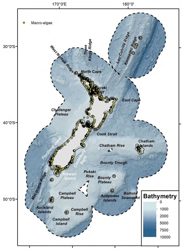
10 Development of a New Zealand Seafloor Community Classification (SCC)2 Biological and environmental datasets (objective 2) 2.1 Study area The study area extended over 4.2 million km2 of the South Pacific Ocean within the New Zealand Territorial Sea (TS) and Exclusive Economic Zone (EEZ) herein referred to as the New Zealand marine environment (≈25 – 57°S; 162°E – 172°W; Figure 2-1). Figure 2-1: Map of the study region. New Zealand Exclusive Economic Zone (EEZ, black dashed line), Territorial Sea (TS, solid black line), water depth and feature names used throughout the text are displayed. Development of a New Zealand Seafloor Community Classification (SCC) 11
2.2 Biological samples
Occurrence records for demersal fish, benthic invertebrates (from coastal/offshore waters and
separately from estuaries and harbours), macroalgae and reef fish were collated from various
sources (Table 2-1). All records were groomed: records located on land, outside the New Zealand EEZ
and/or duplicated within and between databases were removed. Taxonomy was standardised across
datasets and years to the most recent nomenclature (metadata for biological data are provided in
Supplementary materials 1).
Records for each of the groups were separately aggregated to unique locations of different spatial
resolutions (see further information in sections 2.2.1 – 2.2.5). Taxa with ≥ 10 unique sample locations
were retained for the analysis (e.g., as in Stephenson et al. 2018a) because this ensured that there
were sufficient samples to run GF models. All available records were used, regardless of the year
and/or season in which they were collected, to maximise the number of species and samples
available for GF modelling. Following quality control and spatial aggregation, a total of 630,997
records across biotic groups occurring at 39,766 unique locations were retained for final analysis.
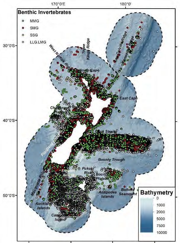
However these were unequally distributed among taxa (Table 2-1) and across the study region
(distribution of samples in Supplementary materials 2: Figure 7-1; Figure 7-2; Figure 7-3; Figure 7-4).
Table 2-1: Summary of information for collated taxa records (after grooming).
Number of Number of
Spatial
Biotic group Source Sampling years taxa (>10 unique
aggregation
occurrences) locations
Demersal fish trawl database (FNZ-NIWA) 1979 – 2016 1 km 317 28,599
Benthic invertebrates NIWA invert database 1896 – 2019 1 km 954
(coastal and offshore)
Te Papa 1966 - 2015 1 km 66
27,274
Auckland Museum 1905 - 2018 1 km 218
trawl database (FNZ-NIWA) 1979 - 2016 1 km 132
Macroalgae NIWA (2019); Te Papa (2012);
Auckland Museum (2019); Duffy
1850 - 2018 250 m 349 3320
(1979 – 2007) and Shears &
Babcock (1999 – 2002)
Reef fish DOC dataset 1986 - 2004 250 m 92 339
Benthic invertebrates NA (see NA (see
OTOT: National Estuary Dataset 2001 – 2017 188
(Estuarine, intertidal) section 2.2.5) section 2.2.5)
2.2.1 Demersal fish
Demersal fish species occurrence and abundance records (n = 391,198) (including information on
research cruise identifier, gear type, date, min and max depth of trawl, and lat/lon) from 1979 – 2016
were extracted from the research trawl database ‘trawl’ (NIWA 2014, 2018). These data were
groomed to only keep those records identified to species level. Species records were spatially
aggregated (based on presence/absence information) to a 1 km grid resolution (e.g., as in
Stephenson et al. 2018a). Species with ≥ 10 unique sample locations at this resolution were retained
for the analysis (e.g., as in Stephenson et al. 2018a). The final demersal fish dataset included
observations for 317 species at 28,599 unique sample locations (Supplementary materials 2: Figure
7-1).
12 Development of a New Zealand Seafloor Community Classification (SCC)2.2.2 Benthic invertebrates (coastal and offshore)
Benthic invertebrate species occurrence records (n = 127,330) (including lat/lon, species name,
collection date, and sampling gear used) from 1896 – 2019 were extracted from trawl (n = 56,841),
NIWA’s Invertebrate Collection database ‘NIWA invert’ (n = 59,144), and databases at Te Papa (n =
2943), and Auckland Museum (n = 8402). These databases also included records for demersal
cephalopod species but for simplicity we refer to them as ‘benthic invertebrates’. In contrast to the
trawl data, which reliably record both species presence and absence of demersal fish, trawl records
do not provide a reliable indication of where benthic invertebrate species do not occur. One way to
overcome this lack of true absence data for the modelling is to use a random selection of points from
the analysis area, treating these as ‘pseudo-absences’. Alternatively, as was undertaken here, the
individual RF species models (generated for GF models) can be constructed using the locations at
which other species not being modelled were present to provide an indication of the ‘relative
absence’, also sometimes referred to as ‘target-group background data’ (Phillips et al. 2009). Better
results can generally be achieved using relative absences compared to randomly selected pseudo-
absences, particularly when the relative absences are drawn from other species records forming part
of the same broad biological group and have been collected using similar methods with the same
sampling biases (Phillips et al. 2009).
Given that the benthic samples were collected using a variety of sampling methods (208 different
gear types), the benthic invertebrate records were grouped into gear categories to reflect
‘catchability’. Many of these gear types were name variants of commonly used sampling gear types,
but for most records, the specific sampling parameters (e.g., mesh size, tow length, etc) were not
recorded. In order to account for both the large number of gear types recorded and the differences
in sampling parameters, gear types were grouped into catchability categories. Catchability was
assumed to be influenced by gear size, deployment area and selectivity (Table 2-2) (Stephenson et al.
2018b).
Table 2-2: Categories used to reflect catchability of sampling gear types. Table modified from (Stephenson
et al. 2018b).
Type Category Description Example
Devonport dredge, box
Small < 1m
corer
Gear size
Medium 1-3m Benthic sled
Large > 3m Otter trawls
Small < 1m Box corer
Deployment area Medium 1m – 1km Beam trawls
Large > 1 km Otter trawls
HS Highly selective Collected by hand
Selectivity
G General Benthic sled
Development of a New Zealand Seafloor Community Classification (SCC) 13Sampling gear types were assigned codes for each of the three catchability types and combined to
yield ‘catchability’ groups (Table 2-3). Out of 18 possible ‘catchability’ groups, six ‘catchability’ groups
occurred in the available invertebrate samples (Table 2-3):
• LLG: Large gear types, deployed over large areas, which were not selective (e.g., otter trawls);
• LMG: Large gear types, deployed over medium-sized areas, which were not selective (e.g., beam
trawls);
• MMG: Medium sized gear types, sampling medium sized areas, which were not selective (e.g.,
benthic sled);
• SMG: Small gear types, sampling medium sized areas, which were not selective (e.g., Devonport
dredge);
• SMHS: Small gear types, sampling medium sized areas, which were highly selective (e.g.,
collected by hand, bottom longline);
• SSG: Small gear types, sampling small areas, which were not selective (e.g., box corer).
Records of LLG and LMG were combined as these catchability groups represent commercial fishing
practices with similar catches of invertebrates likely to be more demersal in nature (i.e., squids). All
records collected from highly selective gear types (e.g., SMHS) were excluded from the analysis,
because methods classified within this group were considered too variable to provide reliable
records of absence (20,010 records were excluded across 412 genera and 2,097 unique locations,
including 190 genera unique to selective methods). Varying degrees of overlap occurred between
genera captured by the different gear type classes in the records retained for analysis - LLG.LMG = 34
% unique genera not shared with other gear types 66% overlap, MMG = 37% unique genera, SMG =
47% unique genera, SSG = 21% unique genera (see Table 2-3 for number of unique genera per gear
type).
Benthic invertebrate records were groomed to keep only those records identified to genus and
species level and within the New Zealand EEZ. These records were aggregated to genus level,
resulting in 127,330 records across 958 genera. Genus records were then spatially aggregated (to
presence - relative absence) at 1 km grid resolution (Supplementary materials 2: Figure 7-2). Records
were aggregated to genus level because this provided a greater number of unique locations than
when records based on species level were aggregated (33,187 vs 28,263 respectively). In addition, at
genus level, benthic invertebrate records were more inclusive across all benthic invertebrate taxa
than records at species level.
14 Development of a New Zealand Seafloor Community Classification (SCC)Table 2-3: Gear type codes used to reflect catchability, number of benthic invertebrate genera > 10
occurrence, number of unique genera > 10 occurrence and number of unique sample locations (see text and
Table 2-2 for Gear type code explanations).
Gear type Number of genera > 10 Number of unique Number of unique
occurrence genera > 10 occurrence locations
LLG.LMG 453 152 23,793
MMG 566 210 1375
SMG 444 208 1883
SSG 43 9 364
All gear types combined 958 958 27,274
SMHS (excluded) 412 190 20,010
2.2.3 Macroalgae
Macroalgae occurrence records were sourced from herbarium records, opportunistic data and
observational datasets. Herbarium records were extracted from databases held at Te Papa
Tongarewa - Museum of New Zealand, Auckland Museum, and NIWA. Opportunistic data were
sourced from citizen science observations of large brown algae collected using iNaturalist (iNaturalist
2019) and verified by photographs as part of an FNZ funded project (ZBD201406). Observational data
were extracted from dive logs collected by Clinton Duffy (DOC) that recorded large brown seaweed
around New Zealand between 1979 and 2007. A second observational dataset was collected by
Shears and Babcock (2007) as part of a research programme on subtidal communities around New
Zealand.
For all datasets, only records that had been identified to species level were used. Occurrence data
were initially restricted to those between 70 m depth and 10 m elevation (including some records on
land) using a New Zealand bathymetry (and elevation) data layer. Records apparently occurring on
land were associated with the closest available marine environmental data. The small number of
records that were obtained from depths between 70 and 200 m depth were checked by macroalgal
experts (W. Nelson and K. Neill) and included in the dataset only if they were considered valid.
Macroalgal presence/absence records were aggregated to 250 m grid resolution. Species with ≥ 10
unique sample locations at this resolution were retained for the analysis. Similarly to the benthic
invertebrate records, ‘target-group background data’ were used as absences. The final macroalgae
dataset consisted of 349 species at 3,320 unique locations (Supplementary materials 2: Figure 7-3).
2.2.4 Reef fish
The relative abundance of reef fishes were obtained from 467 SCUBA dives made around the coast of
New Zealand over an 18-year period from November 1986 to December 2004 (for detailed
methodology see Smith et al. (2013)). These data had previously been groomed and all records were
identified to species level. Records were aggregated (to presence/absence) spatially to a 250 m grid
resolution. Species with ≥ 10 occurrences were retained for the analysis. The final rocky reef fish
dataset included observations of 92 species at 339 unique locations (Supplementary materials 2:
Figure 7-4).
Development of a New Zealand Seafloor Community Classification (SCC) 152.2.5 Benthic invertebrates (Estuarine, Intertidal) The abundance of benthic invertebrates collected from estuaries was retrieved from the National Estuary Dataset (Berthelsen et al. 2020) which was compiled as part of the MBIE-funded Oranga Taiao, Oranga Tangata (OTOT) programme. The dataset is comprised of primarily regional council and unitary authority monitoring data collected from throughout New Zealand. The raw dataset includes data from 70 estuaries, 421 sites and 8305 sampling events collected and analysed by a range of organisations. On average, there were 5.8 sample sites per estuary across 14 councils. All datapoints were collected from the intertidal. Between 3 and 15 replicates were collected at each sampling location, with the maximum sampled area at each location ranging between 1,800 m2 and 10,800 m2. Samples were collected over the period from 2001 to 2017, with variation in the months over which sampling was conducted. This dataset represents some of the best estuarine data available in New Zealand, comprising consistently collected, paired biological and environmental samples. However, sample data were generally collected to investigate change through time rather than to facilitate spatial mapping of environmental and biological patterns. Environmental predictor information for areas outside of sampled locations was very limited and for most estuaries, lacked the resolution required for description of within-estuary variation in environmental and biological character. Therefore, it was not possible to include the estuarine benthic invertebrate data with data from other biotic groups. We provide a separate analysis using this dataset to investigate broad patterns in estuarine bioregionalization. Further details on the methods and results are presented in Supplementary Materials 3 – Estuarine benthic invertebrates. 2.3 Environmental variables New Zealand’s marine environments were described using 33 gridded environmental variables, collated at two resolutions (Table 2-4): a 250 m resolution grid from the coastline to the edge of the Territorial Sea (12 NM from shore), and a 1 km resolution grid from the edge of the Territorial Sea to the edge of the Exclusive Economic Zone (Figure 2-1). Some environmental variable layers were produced at a native resolution of 250 m, e.g., Bathymetry, whereas others required interpolation, e.g., Bottom nitrate (interpolation methods and further information on the environmental layers are available as metadata: Env_pred_metadata – for further information see Supplementary materials 1). Spatial layers were projected using an Albers Equal Area projection centred at 175°E and 40°S (EPSG:9191) now accepted by DOC and Fisheries New Zealand (FNZ) as the standard projection for use with spatial data covering New Zealand’s EEZ (Wood et al. in prep). Environmental variables were selected based on their known influence on growth, survival and distribution of benthic and demersal taxa, and therefore their likely influence on species composition, richness and turnover (e.g., see Leathwick et al. 2006; Compton et al. 2013; Smith et al. 2013; Anderson et al. 2016; Rowden et al. 2017; Stephenson et al. 2018a; Georgian et al. 2019). Several environmental variables showed some co-linearity within records for biotic groups but all levels of co-linearity were considered acceptable (Pearson correlation < 0.9) for tree-based machine learning methods (Elith et al. 2010; Dormann et al. 2013) and more specifically GF modelling (Ellis et al. 2012). The final environmental variables used for GF modelling were selected through a model tuning process which aimed to maximise model fit (see section 3.1). Twenty environmental variables were selected for GF modelling for all biotic groups (grey rows, Table 2-4). In most cases, the inclusion of many variables is avoided because they generally only provide minimal improvement in predictive 16 Development of a New Zealand Seafloor Community Classification (SCC)
accuracy and complicate interpretation of model outcomes (Leathwick et al. 2006). However, here,
the interpretation of model outcomes (i.e., the drivers of distribution) was of secondary interest, the
primary focus being on maximising the predictive accuracy of the model. Values for environmental
variables were derived for each taxon record location by overlay onto the environmental predictor
layers using the “raster” package in R (Hijmans & van Etten 2012). For demersal fish and benthic
invertebrate records this was undertaken using 1 km grid resolution environmental variables
(including in areas where information was available at a 250 m grid resolution in order to match the
spatial scale at which these were sampled), whereas environmental values for reef fish and
macroalgae records were extracted from the 250 m grid resolution environmental variables.

Development of a New Zealand Seafloor Community Classification (SCC)                                 17
Table 2-4:     Spatial environmental predictor variables used for the Gradient Forest analyses. Environmental variables are ordered alphabetically. Environmental variables used
in the final GF models are highlighted in grey.

                                   Temporal                                                                                Native
 Abbreviation      Full name                                                 Description                                                       Units              Source
                                     range                                                                               Resolution
                                              Depth at the seafloor was interpolated from contours generated from
Bathy           Bathymetry        Static      various sources, including multi-beam and single-beam echo sounders, 250 m              m                Mitchell et al. (2012)
                                              satellite gravimetric inversion, and others (Mitchell et al., 2012).
                                              One-year mean value of friction velocity derived from (1) hourly
                                              estimates of surface wave statistics (significant wave height, peak wave
                Benthic
                                  1/7/2017-   period) from outputs of the NZWAVE_NZLAM wave forecast, at 8-km                                          Swart (1974); updated in
Beddist         sediment                                                                                               250 m          ms-1
                                  30/6/2018   resolution, (2) median grain size (d50), at 250 m resolution, (3) water                                  2019
                disturbance
                                              depth, at 25-m resolution. Benthic sediment disturbance from wave
                                              action was assumed to be zero where depth ≥ 200m.
                                              Annual average water nitrate concentration at the seafloor (using NZ
                                              bathymetry layer) based on methods from Dunn et al. 2002. The
                                              oceanographic data used to generate these climatological maps were        approx. 41
BotNi           Bottom nitrate    Static      computed by objective analysis of all scientifically quality-controlled   km (1/2       umol l-1         NIWA, unpublished
                                              historical data from the Commonwealth Scientific and Industrial           degree)
                                              Research Organisation (CSIRO) Atlas of Regional Seas database
                                              (CARS2009, 2009).
                                              Annual average water oxygen concentration at the seafloor (using NZ       Approx. 41
                Dissolved oxygen
BotOxy                           Static       bathymetry layer) based on methods from Dunn et al. 2002.                 km (1/2       ml l-1           NIWA, unpublished
                at depth
                                              Oceanographic data from CARS2009 (2009).                                  degree)
                Oxygen                                                                                                  Approx. 41
BotOxySat       saturation at     Static      Annual average oxygen saturation at the depths.                           km (1/2       umol l-1         NIWA, unpublished
                depth                                                                                                   degree)
                                              Annual average water phosphate concentration at the seafloor (using       Approx. 41
                Bottom
BotPhos                           Static      NZ bathymetry layer) based on methods from Dunn et al. 2002.              km (1/2       umol l-1         NIWA, unpublished
                phosphate
                                              Oceanographic data from CARS2009 (2009).                                  degree)
                                              Annual average water salinity concentration at the seafloor (using NZ     Approx. 41
BotSal          Salinity at depth Static      bathymetry layer) based on methods from Dunn et al. 2002.                 km (1/2       psu              NIWA, unpublished
                                              Oceanographic data from CARS2009 (2009).                                  degree)

18                                                                                                           Development of a New ZealandSeafloor Community Classification (SCC)
Temporal Native
Abbreviation Full name Description Units Source
range Resolution
Annual average water silicate concentration at the seafloor (using NZ Approx. 41
BotSil Bottom silicate Static bathymetry layer) based on methods from Dunn et al. 2002. km (1/2 umol l-1 NIWA, unpublished
Oceanographic data from CARS2009 (2009). degree)
Annual average water temperature at the seafloor (using NZ bathymetry Approx. 41
Temperature at
BotTemp Static layer) based on methods from (Ridgway et al. 2002). Oceanographic km (1/2 °C km-1 NIWA, unpublished
depth
data from (CARS2009 2009). degree)
Terrain metrics were calculated using an inner annulus of 12 km and a
radius of 62 km using the NIWA bathymetry layer in the Benthic Terrain
BPI_broad BPI_broad Static Modeler in ArcGIS 10.3.1.1 (Wright et al. 2012). Bathymetric Position 250 m m NIWA, unpublished
Index (BPI) is a measure of where a referenced location is relative to the
locations surrounding it.
Terrain metrics were calculated using an inner annulus of 2 km and a
radius of 12 km using the NIWA bathymetry layer in the Benthic Terrain
BPI_fine BPI_fine Static Modeler in ArcGIS 10.3.1.1 (Wright et al. 2012). Bathymetric Position 250 m m NIWA, unpublished
Index (BPI) is a measure of where a referenced location is relative to the
locations surrounding it.
The percent carbonate layers for the region were developed from
Percent >30,000 raw sediment sample data compiled in dbseabed, which were
carbonate Static 1 km % Bostock et al. (2019)
carbonate then imported into ArcGIS and interpolated using Inverse Distance
Weighting (Bostock et al. 2019).
NIWA unpublished, updated
in 2020; Based on
A proxy for the biomass of phytoplankton present in the surface ocean processing described in
4 km (ocean)
Chlorophyll-a July 2002 – (to ~30 m depth). Blended from a coastal Chl-a estimate (quasi-analytic Pinkerton et al. (2016) and
Chl-a 500 m mg m-3
concentration March 2019 algorithm (QAA), local aph*(555)) and the default open-ocean chl-a value updated in Pinkerton et al.
(coastal)
from MODIS-Aqua (v2018.0). (2019). QAA algorithm
detailed in (Lee et al. 2002;
Lee et al. 2009)
NIWA unpublished, updated
Chlorophyll-a
July 2002 – Smoothed magnitude of the spatial gradient of annual mean Chl-a. in 2020; Based on
Chl-a.Grad concentration 500 m Mg m-3 km-1
March 2019 Derived from Chl-a described above. processing described in
spatial gradient
(Pinkerton et al. 2018)
Development of a New ZealandSeafloor Community Classification (SCC) 19Temporal Native
Abbreviation Full name Description Units Source
range Resolution
NIWA unpublished, updated
in 2020; Based on
Total detrital absorption coefficient at 443 nm, including due to
processing described in
coloured dissolved organic matter (CDOM) and particulate detrital 4 km (ocean)
Detrital July 2002 – (Pinkerton et al. 2018).
DET absorption. Estimated using quasi-analytic algorithm (QAA) applied to 500 m m-1
absorption March 2019 Processing for
MODIS-Aqua data, blended with adg_443_giop ocean product (Werdell, (coastal)
adg_443_giop ocean
2019).
product described in
(Werdell 2019).
Mean of the 1993-1999 period sea surface above geoid, corrected from
Dynamic geophysical effects taken for the NZ region. This broadly corresponds to
DynOc 1993-1999 250 m m NIWA, unpublished
oceanography mean surface velocity recorded from drifters in the NZ region (Hadfield
pers comm).
Broadband (400–700 nm) incident irradiance (E m-2 d-1) at the seabed,
averaged over a whole year. Estimated by combining incident irradiance NIWA unpublished, updated
4 km (ocean);
Seabed incident July 2002 – at the sea surface ((Frouin et al. 2012); this table), diffuse downwelling in 2020, based on
Ebed 500 m E m-2 d-1
irradiance March 2019 irradiance attenuation (KPAR; this table) and bathymetric depth at processing described in
(coastal)
monthly resolution. Derived from blended coastal (QAA) and open- Pinkerton et al. (2018)
ocean attenuation products.
Net primary production in the surface mixed layer estimated as the NIWA unpublished, updated
Downward
VGPM model ((Behrenfeld & Falkowski 1997); this table). Export fraction in 2020. Based on
vertical flux of
July 2002 – and flux attenuation factor with depth estimated by refitting sediment processing described in
POCFlux particulate 9 km mgC m-2 d-1
March 2019 trap and thorium-based measurements to environmental data (VGPM, Pinkerton et al. (2016) with
organic matter at
SST) as Lutz et al. (2002), Pinkerton et al. (2016) and using data from new data from Cael et al.
the seabed
Cael et al. (2017). (2018).
The percent gravel layers for the region were developed from >30,000
raw sediment sample data compiled in dbseabed, which were then
Gravel Percent gravel Static 1 km % Bostock et al., 2019
imported into ArcGIS and interpolated using Inverse Distance Weighting
(Bostock et al., 2019).
vertical attenuation of diffuse, downwelling broadband irradiance
NIWA unpublished, updated
Diffuse (Photosynthetically Available Radiation, PAR, 400–700 nm). Merged 4 km (ocean)
July 2002 – in 2020; Based on
Kpar downwelling coastal and open-ocean product based on MODIS-Aqua data. Coastal: 500 m m-1
March 2019 processing described in
attenuation estimated from inherent optical properties (QAA). Ocean: estimated (coastal)
Pinkerton et al. (2018)
from K490 using (Morel et al. 2007).
20 Development of a New ZealandSeafloor Community Classification (SCC)Temporal Native
Abbreviation Full name Description Units Source
range Resolution
The depth that separates the homogenized mixed water above from the NIWA unpublished, updated
denser stratified water below. Based on GLBu0.08 hindcast results using in 2020; (Chassignet et al.
Mixed layer July 2002 – a potential density difference of 0.030 kg m-3 from the surface. Models 2007; Wallcraft et al. 2009;
MLD 9 km m
depth March 2019 used are: (1) hycom: from day 265 (2008) to present; (2) fnmoc: from Metzger et al. 2010); Data:
day 169 (2005) to present; (3) soda: from day 249 (1997) to end of 2004; orca.science.oregonstate.ed
(4) tops: from day 001 (2005) to 225 (2010). u
The percent mud layers for the region were developed from >30,000
raw sediment sample data compiled in dbseabed, which were then
Mud Percent mud Static 1 km % Bostock et al., 2019
imported into ArcGIS and interpolated using Inverse Distance Weighting
(Bostock et al., 2019).
The difference between the measured dissolved oxygen concentration Approx. 41
Apparent oxygen
OxyUt and its equilibrium saturation concentration in water with the same km (1/2 umol l-1 NIWA, unpublished
utilization
physical and chemical properties. degree)
Photo- Daily-integrated, broadband, incident irradiance at the sea-surface
July 2002 – NIWA unpublished, updated
PAR synthetically based on day length, solar elevation and measurements of cloud cover 4 km E m-2 d-1
March 2019 in 2020; Frouin et al. (2012)
active radiation from ocean colour satellites (Frouin et al. 2012).
NIWA unpublished, updated
Particulate in 2020; Based on
backscatter at Optical particulate backscatter at 555 nm estimated using blended processing described in
4 km (ocean)
555 nm July 2002 – coastal and ocean products. Coastal: QAA v5 product bbp555 from Pinkerton et al. (2018).
PB555nm 500 m m-1
(previously used March 2019 MODIS-Aqua data. Ocean: bbp_555_giop ocean product (Werdell 2019). Processing for
(coastal)
to generate Result calculated as long-term (2002–2017) average. bbp_555_giop ocean
'turbidity') product described in
Werdell (2019).
Locations of subtidal rocky reefs inferred from navigational charts
Presence /
Reef Rocky reefs Static (Smith et al., 2013). Polygon data converted to raster grids based on > polygon data DOC
absence of reef
50% of polygon in cell.
Roughness of the seafloor calculated as the as the variation in three-
dimensional orientation of grid cells within a neighborhood. Vector NIWA, unpublished data,
Rough Roughness Static 250 m m
analysis is used to calculate the dispersion of vectors normal updated in 2019
(orthogonal) to grid cells within the specified neighbourhood.
Development of a New ZealandSeafloor Community Classification (SCC) 21Temporal Native
Abbreviation Full name Description Units Source
range Resolution
The percent sand layers for the region were developed from >30,000
raw sediment sample data compiled in dbseabed, which were then
sand sand Static 1 km % Bostock et al., 2019
imported into ArcGIS and interpolated using Inverse Distance Weighting
(Bostock et al., 2019).
Annual
Smoothed difference in seafloor temperature between the three
amplitude of sea NIWA, unpublished data,
SeasTDiff Static warmest and coldest months. Providing a measure of temperature 250 m °C km-1
floor updated in 2018
amplitude through the year.
temperature
NA;
Mud;
Muddy gravel;
Muddy sandy
gravel;
Classification of Mud, Sand and Gravel layers (this table) using the well-
Sediment established (Folk et al. 1970) classification. Subtidal rocky reefs (this sand; NIWA unpublished, updated
Sed.class Static 1 km
classification table) were incorporated. This classification provides a broad measure Gravely mud; in 2020
of hardness Mud – Rock. Gravelly sandy
mud;
Gravelly sand;
Gravel;
Rock
Bathymetric slope was calculated from water depth and is the degree NIWA, unpublished,
Slope Slope Static 250m °
change from one depth value to the next. updated in 2019
NIWA unpublished, updated
1981-2018 in 2020; Coastal based on
Blended from OI-SST (Reynolds et al., 2002) ocean product and MODIS- 0.25° (ocean)
Sea surface (ocean) processing described in
SST Aqua SST coastal product. Long-term (2002–2017) average values at 250 1 km °C
temperature 2002-2018 Pinkerton et al. (2018).
m resolution. (coastal)
(coastal) Ocean: (Reynolds et al.
2002)
22 Development of a New ZealandSeafloor Community Classification (SCC)Temporal Native
Abbreviation Full name Description Units Source
range Resolution
1981-2018 Smoothed magnitude of the spatial gradient of annual mean SST. This
Sea surface 0.25° (ocean)
(ocean) indicates locations in which frontal mixing of different water bodies is NIWA unpublished, updated
SSTGrad temperature 1 km °C km-1
2002-2018 occurring (Leathwick et al. 2006).Derived from SST described above at in 2020
gradient (coastal)
(coastal) two resolutions and merged.
Indicative of total
Indicative of total suspended particulate matter concentration. Based
suspended
Suspended on SeaWiFS ocean colour remote sensing data (Pinkerton & Richardson
particulate NIWA unpublished, updated
SuspPM particulate 2005); modified Case 2 atmospheric correction (Lavender et al. 2005); 4 km
matter in 2020; Pinkerton (2016)
matter modified Case 2 inherent optical property algorithm (Pinkerton et al.
concentration (g
2006).
m-3)
Maximum depth-averaged (NZ bathymetry) flows from tidal currents
calculated from a tidal model for New Zealand waters (Walters et al.
2001). Tidal constituents (magnitude A and phase phi, represented as Walters et al., 2001; NIWA
Tidal Current
TC 2009 - real and imaginary parts X + iY = A*exp(i*phi)) for sea surface height and 250 m ms-1 unpublished, updated in
speed
currents (8 components) were taken from the EEZ tidal model, on an 2020
unstructured mesh at variable spatial resolution. The complex
components were bilinearly interpolated to the output grid.
Residuals from a GLM relating temperature to depth using natural
Temperature 1/7/2017-
TempRes splines – this highlights areas where average temperature is higher or 250 m °C Leathwick et al. (2006)
residuals 30/6/2018
lower than would be expected for any given depth.
Net primary
Daily production of organic matter by the growth of phytoplankton in Behrenfeld & Falkowski
production by
the surface mixed layer, net of phytoplankton respiration. Estimated at (1997);
the vertically- July 2002 –
VGPM monthly resolution based on satellite observations of chl-a, PAR and 9 km mgC m-2 d-1
generalised March 2019 NIWA unpublished, updated
SST, and model-derived estimates of mixed-layer depth, using the
production in 2020
vertically-generalised production model (Behrenfeld & Falkowski, 1997).
model
Development of a New ZealandSeafloor Community Classification (SCC) 233 Development of a Gradient Forest environmental classification
(Objective 3)
GF models were used to analyse and predict spatial patterns of compositional turnover for species in
each of four biotic groups: demersal fish, reef fish, benthic invertebrates, and macroalgae, following
analytical methods described in Ellis et al. (2012); Pitcher et al. (2012). These four turnover models
were then combined to derive estimates of compositional turnover along each of the environmental
gradients. Associated uncertainty estimates were also produced. Finally, the combined compositional
turnover was hierarchically classified to a 30-, 50-, 75-, and 100-group level (i.e., inferred community
groups) across the New Zealand TS and EEZ (Figure 3-1). Here we describe in detail the 75-group
classification, which we refer to as the ‘New Zealand Seafloor Community Classification’ (SCC). All
modelling was undertaken in R (R Core Team 2020). Metadata for all data used in the models, R
code, and output files are provided in Supplementary Materials 1.
3.1 Methods
3.1.1 Estimating compositional turnover
For each biotic group (demersal fish, macroalgae and reef fish) and for the different benthic
invertebrate sampling gear types (LLG.LMG, MMG, SMG and SSG) GF models were fitted using the
‘extendedForest’, (Liaw & Wiener 2002) and ‘gradientForest’ (Ellis et al. 2012) R packages (Figure 3-
1). GF models were fitted with 500 trees and default settings for the correlation threshold used in the
conditional importance calculation of environmental variables. For each of the 7 GF models, we
extracted information on the predictive power of the individual RF models (R2f for each taxon
measured as the proportion of out-of-bag variance explained) (Ellis et al. 2012) and the importance
of each environmental variable (R2 assessed by quantifying the degradation in performance when
each environmental variable was randomly permuted1 (Pitcher et al. 2012). The environmental
variables used in each GF model were selected to maximise the number of taxa effectively modelled
(i.e., taxa with R2f > 0) and increase model fits for the most poorly modelled taxa (i.e., taxa with low
R2f).
GF aggregates the values of the tree-splits from the RF models for all taxon models with positive fits
(R2f > 0) to develop empirical distributions that represent taxa compositional turnover along each
environmental gradient (Ellis et al. 2012; Pitcher et al. 2012). The turnover function is measured in
dimensionless R2 units, where taxa with highly predictive random forest models (high R2f values) have
greater influence on the turnover functions than those with low predictive power (lower R2f). The
shapes of these monotonic turnover curves describe the rate of compositional change along each
environmental predictor; steep parts of the curve indicate fast assemblage turnover, and flatter parts
of the curve indicate more homogenous regions (Ellis et al. 2012; Pitcher et al. 2012; Compton et al.
2013).
The use of the dimensionless R2 to quantify compositional turnover enables information from
multiple taxa to be combined, even if that information comes from different sampling devices,
surveys or regions (Ellis et al. 2012). In the first instance, the compositional turnover functions from
each of the benthic invertebrate gear type GF models were combined using the
‘combinedGradientForest()’ function to provide a combined benthic invertebrate GF model (herein
1Note that R2 described by Pitcher et al., 2012 and Ellis et al., 2011 refers to a unitless measure of cumulative importance and should not
be confused with the more commonly used R-squared (R2) denoting coefficient of determination.
24 Development of a New ZealandSeafloor Community Classification (SCC)You can also read