Sea surface temperature fronts in the California Current System from geostationary satellite observations
←
→
Page content transcription
If your browser does not render page correctly, please read the page content below
JOURNAL OF GEOPHYSICAL RESEARCH, VOL. 111, C09026, doi:10.1029/2006JC003541, 2006
  Click
  Here
    for
 Full
Article

Sea surface temperature fronts in the California Current System
from geostationary satellite observations
Renato M. Castelao,1,2 Timothy P. Mavor,3,4 John A. Barth,1,2 and Laurence C. Breaker5
Received 15 February 2006; revised 12 May 2006; accepted 14 June 2006; published 23 September 2006.

[1] Sea surface temperature (SST) fronts are determined for the 2001–2004 time period
from Geostationary Operational Environmental Satellites (GOES) data in the California
Current System (CCS). The probability of detecting a SST front at an individual pixel
location in the CCS is presented as a bi-monthly climatology. Fronts clearly indicate the
seasonal evolution of coastal upwelling, as well as meanders and filaments that are often
linked with irregularities in coastline geometry. Winter is characterized by low frontal
activity along the entire coast. Fronts first appear close to the coast during spring,
particularly south of Cape Blanco, where upwelling favorable winds are already persistent.
The area of high frontal activity continues to increase during summer, especially
between Monterey Bay and Cape Blanco, extending more than 300 km from the coast.
The region with high frontal activity widens at 2.6 km day 1. Off northern Baja
California, a band with persistent fronts is found close to the coast year-round, but there
is no evidence of a seasonal widening of the area of higher activity. During fall, the
weakening of upwelling favorable winds leads to a gradual decrease in frontal activity.
An empirical orthogonal function (EOF) decomposition reveals the development of SST
fronts associated with seasonal upwelling for locations north of Monterey Bay, with
less summer intensification to the south. The first appearance of fronts close to the coast
during spring and the occurrence of the fronts offshore later in the season are represented
by additional statistically significant EOF modes.
Citation: Castelao, R. M., T. P. Mavor, J. A. Barth, and L. C. Breaker (2006), Sea surface temperature fronts in the California
Current System from geostationary satellite observations, J. Geophys. Res., 111, C09026, doi:10.1029/2006JC003541.

1. Introduction                                                                great importance to the productivity of the waters off the
                                                                               coast, because the rising water brings nutrients to the
  [2] The California Current System (CCS) is the eastern
                                                                               euphotic zone [Sverdrup et al., 1942], which is reflected
boundary current of the North Pacific ocean off the U.S. and                   in the distribution of phytoplankton [Sverdrup and Allen,
Mexico west coasts. Its northern extent is marked by the                       1939]. The CCS is thus nutrient-rich, sustaining a highly
southward branch of the bifurcating North Pacific Current                      productive food web [Walsh, 1977]. During winter, the wind
(also known as West Wind Drift) off Washington, and it                         forcing is strongly downwelling-favorable in the northern
extends south to Baja California. A complex current struc-                     region [Huyer, 1983; Bakun and Nelson, 1991], particularly
ture is present in the region, including the equatorward                       off Oregon and Washington, but as far south as 35°N during
California Current, the poleward California Undercurrent,                      storms.
and the Inshore Countercurrent (the Inshore Countercurrent                       [4] There have been several observational efforts in the
is often called the Davidson Current in certain locations).                    CCS over the last 20 years or so, which dramatically
Detailed reviews of the circulation in the CCS can be found                    changed our view of the region. Originally, the CCS
in Hickey [1979, 1998] and Huyer [1983].                                       was viewed as a very broad and weak equatorward flow
  [3] Prevailing winds during summer are equatorward                           [Wooster and Reid, 1963; Hickey, 1979]. Synoptic surveys
throughout the region [Huyer, 1983], resulting in offshore                     have shown that this can be quite misleading [Huyer et al.,
Ekman transport and upwelling along the coast. This is of                      1998], and intense jets with core velocities of 0.5 –0.8 m s 1
                                                                               lying offshore of the continental margin are frequently
   1
     College of Oceanic and Atmospheric Sciences, Oregon State                 found [Kosro and Huyer, 1986; Chelton et al., 1987; Kosro
University, Corvallis, Oregon, USA.                                            et al., 1991; Strub et al., 1991; Barth et al., 2005].
   2
     Cooperative Institute for Oceanographic Satellite Studies, Oregon State   The California Current is often concentrated in a narrow,
University, Corvallis, Oregon, USA.                                            meandering jet embedded in a rich eddy field [e.g., Strub
   3
     National Environmental Satellite, Data and Information Service,
NOAA, Camp Springs, Maryland, USA.                                             and James, 1995; Kelly et al., 1998; Brink et al., 2000]. The
   4
     STG, Inc., Reston, Virginia, USA.                                         recent availability of long-term surface drifter and satellite
   5
     Moss Landing Marine Laboratories, Moss Landing, California, USA.          sea level data allow for descriptions of the seasonal cycle of
                                                                               the California Current and eddy fields [Kelly et al., 1998;
Copyright 2006 by the American Geophysical Union.                              Strub and James, 2000, hereafter SJ2000].
0148-0227/06/2006JC003541$09.00

                                                                        C09026                                                        1 of 13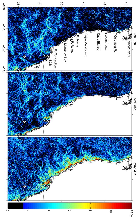
C09026                                 CASTELAO ET AL.: SST FRONTS IN THE CCS                                            C09026

  [5] Field data from summer off northern California often        of several months or more makes satellite measurements
show the jet flowing along a sharp gradient in sea surface        ideal for observing the evolution of SST fronts. Despite the
temperature (SST) [Kelly, 1983; Swenson et al., 1992;             extensive literature on the circulation in the CCS, few
SJ2000]. Huyer et al. [1998] showed that the baroclinic           studies have addressed the seasonal evolution of thermal
velocity extends down to 200 m and more, without signif-          fronts. Breaker and Mooers [1986] used AVHRR (Ad-
icant changes in the position and orientation of the jet,         vanced Very High Resolution Radiometer) imagery to
although decreasing in intensity by a factor of 5 or more.        follow the seasonal migration of upwelling-related fronts
Thus, the locations of the SST fronts are a relatively good       offshore. They found that off Point Sur (36°N), the major
proxy for the location of the jet. However, this is not always    upwelling front migrates offshore during the spring and
true, as the SST reflects not only the mesoscale velocity         summer probably due to Ekman transport over periods of
field, but also other superficial processes of short duration     days-to-weeks, but consistent with Rossby wave dynamics
and small scales, such as internal waves, turbulence, and         over longer periods. Castelao et al. [2005] used one year of
inhomogeneities in surface heating and mixing [Huyer et           Geostationary Operational Environmental Satellites (GOES)
al., 1998]. One of the most important aspects of ocean            SST frontal data to describe the seasonal evolution of the
fronts is that they are characterized by convergent flow at       fronts focusing on flow-topography interactions. Their
the surface [Bowman, 1978]. For this reason, fronts are           study region was restricted to Oregon and northern Cal-
regions that are rich in biological productivity. Free floating   ifornia. In the present study, we use a 4-year long time series
biota are drawn into frontal zones due to the prevailing          of GOES SST data to identify zones of persistent frontal
convergent flow, a process that in time can lead to a fully       activity and to describe their evolution throughout the year
developed food chain as fish at higher trophic levels are         in the whole CCS. The use of data from a geostationary
likewise attracted to these regions in search of food.            satellite is a great advantage over using polar-orbiting
  [6] Frontogenesis in the surface layer of the ocean on          satellite infrared data, since the study region tends to be
time scales of a week or less results primarily from              cloudy in all seasons, and only relatively few clear AVHRR
differential horizontal and vertical temperature advection        images are generally obtained [see Chelton and Wentz,
[Roden and Paskausky, 1978]. In the CCS, one cause of             2005, Figure 3]. Using the GOES-derived frontal data
ocean fronts is coastal upwelling, which is a dominant            allowed for much more reliable statistics.
physical process within about 50 km of the coast from
spring to early fall. Because upwelling fronts tend to slope      2. Data and Methods
in the same direction as the cross-shelf topography, they are
often referred to as prograde fronts [Mooers et al., 1978].         [8] Maps of ocean fronts in the CCS have been produced
Small scale fronts may be associated with estuarine/river         using infrared (IR) imagery from the imager on the GOES-10
discharge. Near the coast in shallow water where the              geostationary satellite. The imager on GOES-10 has im-
influence of bottom topography may be strong, fronts can          proved spatial resolution compared to data from previous
be associated with major bathymetric features, particularly       geostationary satellites [Menzel and Purdom, 1994]. GOES
along the continental margin [Holladay and O’Brien, 1975].        satellites, because of their geostationary orbit, can acquire
Further from shore, upwelled waters may be more the result        several images per day, providing far more opportunities to
of positive wind stress curl that leads to divergent flow near    obtain cloud-free coverage of the study area than could be
the ocean surface, thus controlling Ekman pumping and             acquired from polar-orbiting satellites that sample a given
associated vertical advection. Negative wind stress curl          location twice each day. With respect to the CCS, persistent
(Ekman convergence) is characteristic of the region even          cloud cover has limited the utility of polar-orbiting satellite
farther from shore [Bakun and Nelson, 1991] (D. B. Chelton        coverage [Breaker et al., 2005; Chelton and Wentz, 2005].
et al., Summertime coupling between sea surface tempera-            [9] The GOES-10 geostationary satellite is positioned
ture and wind stress in the California Current System,            above the equator at 135°W, providing spatial coverage of
submitted to Journal of Physical Oceanography, 2006). That        a region that extends from 45°S to 60°N, and from 90°W to
implies favorable conditions for formation of fronts and          180°W. Hourly derived SSTs from the GOES satellites,
convergent patches of recently upwelled water [Bakun and          operated by National Oceanic and Atmospheric Adminis-
Nelson, 1977]. Beyond the region directly influenced by           tration’s (NOAA) National Environmental Satellite, Data
coastal upwelling lies the Coastal Transition Zone [Brink         and Information Service (NESDIS), became routinely avail-
and Cowles, 1991], a region inhabited by long filaments of        able in 2000. Multichannel brightness temperatures at 3.9,
cold water that often originate closer to the coast and, in       11, and 12 microns are retrieved from the imager on the
some cases, originate at coastal capes that may serve as          GOES satellites using an operational algorithm to produce
upwelling centers. These features possess frontal boundaries      SST fields on an hourly basis at approximately 5 km
that separate them from the surrounding offshore waters.          resolution. Utilization of various wavelengths in the multi-
Wave-like instabilities along major upwelling boundaries          channel SST and cloud-clearing algorithms produce SST
can lead to eddy formation [Breaker and Mooers, 1986],            retrievals with acceptable accuracy when compared to buoy
which are known to play an important frontogenetic role           observations (E. Maturi, personal communication, 2005).
[Fedorov, 1986].                                                  By using a multichannel retrieval algorithm, the effects of
  [7] Looking at SST fronts in the CCS is particularly            atmospheric moisture are also removed. A cloud screening
interesting, as it has been hypothesized that the ultimate        algorithm using the multi-channel approach of Wu et al.
source of energy in the jet in the region is the formation of     [1999] is used to identify picture elements (pixels) in the
the density (or temperature) front close to the coast             image that are obscured by cloud. However, marine stratus
(SJ2000). High spatial and temporal resolution over periods       along the U.S. west coast is often similar in temperature to

                                                             2 of 13
C09026                                 CASTELAO ET AL.: SST FRONTS IN THE CCS                                          C09026

                                                                 rithm are dependent on the choice of the color palette and
                                                                 scaling used to construct Figure 1. Comparisons of fronts
                                                                 detected with gradient magnitude images show the chosen
                                                                 threshold values capture most of the main fronts in the CCS.
                                                                 Due to the large spatial and temporal variability in cloud
                                                                 cover, comparisons of frontal occurrences between different
                                                                 regions and time periods is often difficult, since each region
                                                                 is, in general, sampled at different times. This is especially
                                                                 important when making seasonal comparisons of composite
                                                                 frontal images, since the amount of cloudiness is variable in
                                                                 space and time. Following Ullman and Cornillon [1999]
                                                                 and Mavor and Bisagni [2001], for each frontal image, we
                                                                 take the number of times a particular pixel qualifies as a
                                                                 front and divide this value by the number of times that the
                                                                 pixel was clear during that time period, yielding a proba-
                                                                 bility of detecting a front (PDF). Since SST gradients are
                                                                 weak during winter, although fronts may occur, they are
                                                                 more difficult to detect using SST as a tracer. Because of the
                                                                 processing methods employed, it was not possible to extract
                                                                 frontal activity within the first 30 km of the coast.

                                                                 3. Seasonal Evolution of SST Fronts
                                                                   [11 ] The climatological frontal activity in the CCS
                                                                 presents substantial variability, both spatially and temporal-
                                                                 ly (Figures 2a and 2b and Figures 3a and 3b).
                                                                 3.1. January-February
                                                                   [12] At the beginning of the year, during Jan-Feb, the
                                                                 PDF averaged over the entire CCS is at a minimum
Figure 1. GOES-derived daily averaged SST (°C) from
                                                                 (Table 1). There is a roughly 100– 150 km wide band close
25 August 2001. Clouds are shown in white. Black dots
                                                                 to the coast to the north of Point Conception (34°N) with
mark the location of fronts found by the edge-detection
                                                                 nearly zero PDF (Figure 2a). That pattern is only broken to
algorithm. The 200-m isobath is shown. SCB: Southern
                                                                 the north of the Columbia river mouth (46°N), where the
California Bight, NBC: Northern Baja California.
                                                                 PDF increases significantly. During winter, the prevailing
                                                                 winds and coastal currents off Oregon and Washington are
the underlying SST, and thus the influence of cloud cover        northward. The plume from the Columbia river is usually
may not always be removed [Breaker et al., 2005].                observed north of the river mouth [Hickey, 1989, 1998;
  [10] After cloud screening, daily-averaged SST fields are      Garcı́a Berdeal et al., 2002], which could explain the
calculated for the period from 2001 to 2004, based on 24         localized increase in the PDF observed there. The plume
hourly GOES SST fields. A Sobel gradient operator is used        creates a shallow layer which can become warmer than
to estimate the sea surface temperature gradient magnitude       surrounding waters due to surface heating. Also, river waters
(SSTGM). SST fields are then processed by an edge-               during winter are generally colder than oceanic waters. Both
detection algorithm [Canny, 1986] to identify SST fronts.        processes would lead to enhanced PDF. The wintertime PDF
The SST field is first smoothed, followed by the computa-        is relatively high in the Southern California Bight (SCB),
tion of the gradient vector. The algorithm then tracks in the    between 28° and 35°N offshore, and along a thin band off the
direction of the gradient, suppressing any pixel that is not a   Mexican coast, where the climatological wind forcing is
local maximum (nonmaximum suppression). The thresh-              upwelling favorable even during the winter. These areas also
olding in the edge-detection algorithm is done with hyster-      have local intensification in the SSTGM (Figure 3a), but
esis. The algorithm first looks for pixels with gradient         values are generally small.
magnitude larger than a threshold T1. These pixels are
flagged as frontal pixels. Then, the algorithm tracks along      3.2. March-April
a front crest (i.e., perpendicular to the gradient), flagging      [13] In late winter and early spring (Mar-Apr), the PDF is
pixels as frontal pixels until the gradient magnitude falls      still very low north of Cape Mendocino, but increases
below a smaller threshold T2. This helps to ensure that noisy    considerably south of it. This is consistent with the wind
edges are not broken up into multiple edge fragments.            stress seasonal cycle and the seasonal development of
Thresholds employed are 0.006 and 0.0015°C km 1. Note            upwelling. The climatological winds in the northern part
that the Canny method involves significantly smoothing the       of the domain are very weak in early spring [Strub et al.,
SST field before computing the gradients. A typical              1987], but upwelling favorable winds intensify south of
declouded SST image overlain with the detected fronts is         Cape Mendocino (41°N) [Huyer, 1983]. This suggests
shown in Figure 1. Note that some of the apparent fronts in      coastal upwelling is an important mechanism for generation
offshore waters not detected by the edge-detection algo-         of the fronts. High values are found between Point Arena

                                                            3 of 13
C09026
4 of 13
CASTELAO ET AL.: SST FRONTS IN THE CCS
Figure 2a. Seasonal probability of detecting a SST front (%) from January to June derived from GOES satellite data, 2001
through 2004. The probability is the ratio of the number of the times a pixel contained a front to the number of times the
pixel was cloud-free. Probabilities 1.5% are not shown, and 12% are shown in dark red in order to reveal as much of the
horizontal structure as possible. The 200-m isobath is shown. SCB: Southern California Bight, NBC: Northern Baja
California.
C09026C09026
5 of 13
CASTELAO ET AL.: SST FRONTS IN THE CCS
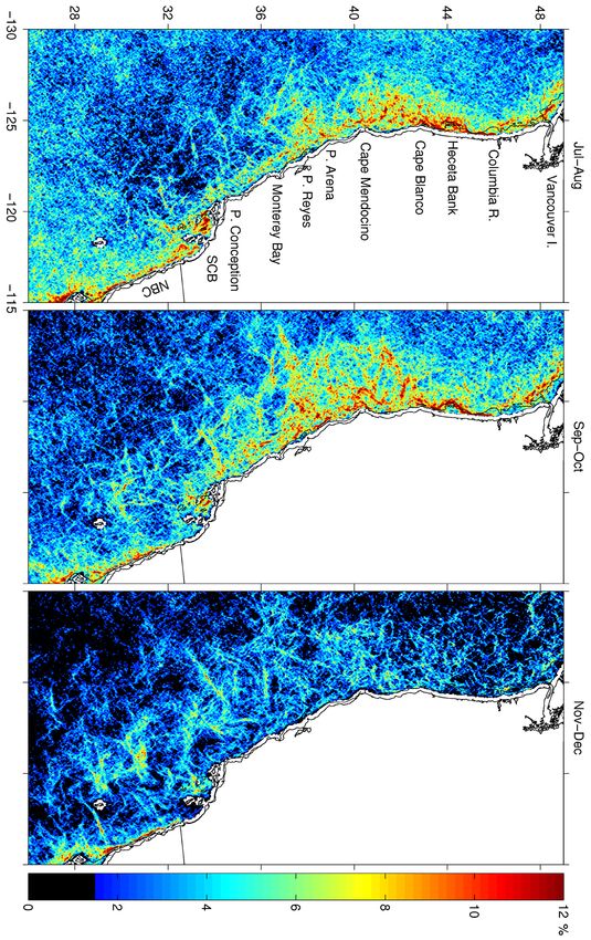
Figure 2b. Seasonal probability of detecting a SST front (%) from July to December derived from GOES satellite data,
2001 through 2004. The probability is the ratio of the number of the times a pixel contained a front to the number of times
the pixel was cloud-free. Probabilities 1.5% are not shown, and 12% are shown in dark red in order to reveal as much of
the horizontal structure as possible. The 200-m isobath is shown. SCB: Southern California Bight, NBC: Northern Baja
California.
C09026C09026
6 of 13
CASTELAO ET AL.: SST FRONTS IN THE CCS
Figure 3a. Mean seasonal SST gradient magnitude (°C km 1) from January to June derived from GOES satellite data,
2001 through 2004. Gradient magnitudes 0.009°C km 1 are not shown. The black contour is the 200-m isobath. SCB:
Southern California Bight, NBC: Northern Baja California.
C09026C09026
7 of 13
CASTELAO ET AL.: SST FRONTS IN THE CCS
Figure 3b. Mean seasonal SST gradient magnitude (°C km 1) from July to December derived from GOES satellite data,
2001 through 2004. Gradient magnitudes 0.009 °C km 1 are not shown. The black contour is the 200-m isobath. SCB:
Southern California Bight, NBC: Northern Baja California.
C09026C09026 CASTELAO ET AL.: SST FRONTS IN THE CCS C09026
Table 1. Overall Averaged Probability of Detecting a Front (%) in A somewhat similar feature is also observed off Point
the CCS, 2001 Through 2004 Conception, although with smaller probability values. Off
northern Baja California, the increase in the area with high
Jan-Feb Mar-Apr May-Jun Jul-Aug Sep-Oct Nov-Dec
PDF and SSTGM close to the coast is less evident than
2.37 2.47 3.22 4.54 4.21 2.86 between 34° and 43°N.
3.4. July-August
(39°N) and Point Reyes (38°N), south of Monterey Bay [16] The PDF field evolves considerably from late spring
(36°N), in the SCB and off northern Baja California, where to summer. The highest overall PDF in the CCS is found in
local intensifications of the SSTGM are also found. The the Jul-Aug composite (Table 1). North of Cape Blanco,
band with high values (both for PDF and SSTGM) off values increase substantially compared with May-Jun (PDF
northern Baja California is very narrow. The PDF in the in excess of 25% in some places) in a band extending 50–
offshore region (more than 200 km from the coast, west of 100 km from the coast. SST images from several years show
Point Conception) decreased compared with Jan-Feb. Using that the upwelling region north of Cape Blanco during
altimeter satellite observations, SJ2000 showed that, al- summer is much narrower than south of it [Strub et al.,
though the velocity variances next to the coast begin to 1991; Barth et al., 2000; SJ2000] (among others), a result
increase during spring, the kinetic energy 400 km offshore supported by in situ data [Barth and Smith, 1998; Barth et
reaches its seasonal minimum. The present results are al., 2000]. The fronts, therefore, occupy roughly the same
consistent with theirs, if we assume that the temperature region for long periods of times, leading to the high PDF
fronts coincide with intensifications in the flow velocities. found there. Over Heceta Bank, the maximum PDF follows
the 200-m isobath, with a region of decreased PDF inshore.
3.3. May-June A detailed analysis of the seasonal evolution of GOES SST
[14] During late spring (May-June), winds become pre- fronts around Heceta Bank is found in Castelao et al.
dominantly upwelling favorable in the entire CCS. This [2005].
leads to the first persistent appearance of SST fronts around [17] As in late spring, the width of the area with high PDF
Cape Blanco (43°N, Figure 2a). A local increase in frontal increases south of Cape Blanco. There is a remarkable
activity is also found around Heceta Bank (44°– 45°N), difference from before, however. In May-Jun, maximum
and from the Columbia river mouth to the Strait of Juan de values south of Cape Blanco were found close to the coast,
Fuca (48°N), although the PDF is much smaller than to the decreasing offshore. This is no longer true in the Jul-Aug
south of Cape Blanco (43°N). In those regions north of climatology. Maximum values are found scattered in a
43°N, the highest PDF is found inshore of the 200-m 200 km wide region, and are smaller in magnitude than
isobath. north of Cape Blanco. Several numerical [e.g., Haidvogel et
[15] South of Cape Blanco, the accumulating input of al., 1991; Batteen, 1997] and laboratory [e.g., Narimousa
energy from the wind to the system leads to the intensifi- and Maxworthy, 1989] modeling studies have shown that
cation of the coastal upwelling jet and the persistent more vigorous meanders and filaments are produced when
occurrence of SST fronts. Maximum values are found in a capes are introduced. Irregularities in the coastline geometry
thin band extending all the way to the SCB, but high values are thus key elements for anchoring upwelling filaments
are found in a much wider and convoluted area compared [Batteen, 1997]. The Cape Blanco region was identified as
with late winter and early spring. The SSTGM map the location where the inshore edge of the California
(Figure 3a) reveals that stronger fronts are found just south Current leaves the coast and develops a meandering jet to
of Cape Blanco and Cape Mendocino, off Point Reyes and the south [e.g., Barth et al., 2000; Batteen et al., 2003],
in the SCB. The increase in the distance from the coast leading to constant shifts in the position of the SST fronts,
where a high PDF and SSTGM are found occurs to the which could explain the smaller PDFs found there. The
south of Cape Blanco. Previous studies have shown that an SSTGM is relatively large upstream of Heceta Bank and
equatorward jet regularly separates from the coast at Cape Cape Blanco, and decreases abruptly south of the cape.
Blanco to become an oceanic jet [Barth and Smith, 1998; SJ2000 suggest conversion of potential energy to eddy
Barth et al., 2000]. It is interesting to note that the area with kinetic energy (EKE) around the core of the jet by instabil-
high PDF suddenly narrows between Cape Mendocino and ity processes as the system moves offshore is an important
Point Arena, before widening again to the south. This may mechanism responsible for weakening the fronts. The
be the signature of a (warm) anticyclonic meander frequently constant shift in the position of the fronts is also certainly
observed west of Point Arena [Lagerloef, 1992; SJ2000] important for weakening the average gradient magnitude
and shown in maps of dynamic height in the CalCOFI south of Cape Blanco. South of Cape Mendocino, the
(California Cooperative Oceanic Fisheries Investigations) region with high PDF narrows again (as in late spring),
data [Wyllie, 1966]. The narrowing of the area with high with the signature of the anticyclone located there intensi-
PDF in the 4-year average supports the observation that the fied. West of Point Arena, high PDF is encountered out to
meander repeatedly appears in different years. Also striking 300– 350 km from the coast, a signature of upwelling
in the late spring PDF map is the localized narrow feature filaments which inhabit the Coastal Transition Zone [Brink
found just off Point Reyes (also seen in the SSTGM map), and Cowles, 1991]. The recurrent anticyclone is apparently
with high values extending for about 170 km from the coast. coupled with recurrent cold upwelling filaments [Lagerloef,
This is presumably associated with the development of cold 1992], which are frequently observed off Point Arena [e.g.,
upwelling filaments, which are frequently observed at that Strub et al., 1991; Swenson et al., 1992; Huyer et al., 1998].
time of the year [e.g., Strub et al., 1991; Barth et al., 2002].
8 of 13C09026 CASTELAO ET AL.: SST FRONTS IN THE CCS C09026
[18] The band of high PDF is considerably narrower similar decrease is also observed in the monthly averaged
south of Monterey Bay. In fact, the width between Monte- altimetric and drifter-derived surface EKE field [Kelly et al.,
rey Bay and Point Conception is approximately equal to the 1998]. Haney et al. [2001] used a numerical model to show
width found in late spring. One of the most remarkable that this rapid decrease can be attributed to the transforma-
features in the Jul-Aug SSTGM field is the region of low tion of upper-ocean baroclinic shear EKE, associated with
values between Monterey Bay and Point Conception. Off- SST fronts via thermal wind, to deeper EKE (i.e., barotrop-
shore of the coastal band (100 km west-southwest of Point ization). Upwelling filaments off Point Arena at this time
Conception), the PDF and the SSTGM are very low. In the extend out to 500 km from the coast. As during early
SCB, the PDF is high. During summer, upwelled water summer, the SSTGM decreases sharply to the south of
from the north is advected into the northern part of the Bight Cape Mendocino.
[Hickey, 1992], while warm water is carried into the [20] In contrast to results north of Monterey Bay, there is
southern part of the Bight by a cyclonic turn of the not a great increase in the width of the area with high PDF
currents (SJ2000), establishing strong temperature fronts south in the SCB and off Baja California. This area is actually
(Figure 3b). Off northern Baja California, fronts are con- characterized by relatively high PDF year-round, with little
centrated close to the coast, particularly in the vicinity of seasonal widening of the area with high PDF. Throughout the
Punta Eugenia (28°N), with a rapid decrease of the PDF in year there is a consistent tendency for a lobe of anticyclonic
the offshore direction. The SSTGM is also higher close to wind curl to penetrate coastward from the offshore region to
the coast, decreasing in the offshore direction. The decrease contact the coast of Baja California around 30°N [Bakun and
in frontal activity in the offshore region off Baja may be Nelson, 1977, 1991], which might help explaining the per-
partially due to increased solar insolation, which partially sistent occurrence of fronts there. Drifter data from Brink et al.
offsets upwelling leading to nearly homogeneous temper- [2000] showed evidence of a strong meandering jet (speeds
atures in the offshore direction [Bakun and Nelson, 1977]. >0.4 m s 1) north of 35°N. The number of drifters embedded
That may have also been affected by the occurrence of a weak in strong jets decreased substantially between 35° and 30°N,
El Niño during 2002 –2003 [Murphree et al., 2003], which becoming nearly nil south of that. Since strong jets often have
tends to decrease upwelling, which in turn decreases insta- an associated surface temperature front (as is frequently the
bilities of alongshore flow and mesoscale activity [Durazo case in the CCS), the PDF and SSTGM climatologies pre-
and Baumgartner, 2002]. It is very clear, however, that the sented here are generally consistent with this interpretation.
offshore extent of the region with stronger fronts increases There is a strong decrease in the PDF in the offshore region
toward the south off northern Baja California. Brink et al. between 35°N and 30°N, and very low values south of that
[2000] used 2 years of drifter data to show that almost all (note that low values in that area are also observed in spring).
drifters that reached as far south as 15°– 25°N turned west- The SSTGM is also small in that area during spring and
ward. The drifters continued westward in the North Equato- summer. High values are only found close to the coast, a
rial Current, and they estimated that the northern edge of the region poorly sampled by the drifters [see Brink et al., 2000,
current was at 25°N. This might explain the increase in the Plate 1].
offshore extent reached by stronger fronts in the southern part [21] The PDF and SSTGM fields during July to October
of the domain shown in Figure 3b during early to mid- suggest the existence of 3 different regions in the CCS
summer, although this region is north of the position of the during summer. The first region extends from halfway
current based on historical observations. between Cape Mendocino and Cape Blanco to Vancouver
Island. Fronts there are frequent, strong, and spatially
3.5. September-October locked within 100 km from the coast. In the second region
[19] Climatological wind forcing is still upwelling favor- (Point Conception to halfway between Cape Mendocino
able over most of the region during Sep-Oct (the exception and Cape Blanco), fronts are frequent, but spread out up to
is north of Cape Blanco during October). Although the 300– 500 km from the coast. The climatological SSTGM is
overall averaged PDF decreases from early-mid summer (by substantially weaker than in the north. In the third region
less than 10%, Table 1), the width of the region with high (south of Point Conception), fronts are strong and frequent,
PDF is at a maximum (Figure 2b). North of the Columbia but restricted to close to the coast.
river mouth, the most persistent location with occurrence of 3.6. November-December
fronts has moved offshore compared to spring, and is [22] November and December are characterized by pre-
located offshore of the 200-m isobath. The width of the dominantly poleward wind forcing north of Cape Men-
area with high PDF also increases around Heceta Bank, but docino, and weakly upwelling favorable winds to the
there is not much change in the location of the highest south. This leads to a rapid decrease in frontal activity
values (i.e., still follows the 200-m isobath). The increase in observed in the CCS. Consistent with the wind forcing, the
the area of frontal activity is most evident from Cape Blanco strongest decrease is observed off the Oregon and Wash-
to Monterey Bay, where high values are found extending ington coasts (Figures 2b and 3b). South of Point Arena/
more than 300 km from the coast. Capes direct flow Point Reyes, a region with higher PDF is found offshore
offshore, and filaments form which also have frontal (127°W, 37°N to 119°W, 28°N), roughly 300 km from
boundaries. This is consistent with results from other years. coast, with smaller probabilities inshore (except for north-
SJ2000 reported that the core of the equatorward flow in ern Baja California, which also has high values in a
October 1993 occurred 300 – 350 km from the coast south of narrow band close to the coast). The SSTGM map presents
43°N, with a convoluted region of cool water farther a similar pattern, although higher values offshore do not
inshore. The PDF decreases rapidly beyond this region. A extend north of 35°N. The offshore maxima in the PDF and
9 of 13C09026 CASTELAO ET AL.: SST FRONTS IN THE CCS C09026
the SSTGM decrease with time, and smaller values are found around the Heceta Bank region, close to the 200-m isobath,
early in the year (Jan-Feb). and on a wider area between Cape Blanco and Cape
Mendocino, although with a somewhat smaller magnitude.
4. Offshore Migration of the Fronts The seasonal variability in the PDF is considerably smaller
to the south. Strub et al. [1987] also observed a strong
[23] Breaker and Mooers [1986] showed that the along- decrease in the magnitude of the seasonal cycle of several
shore mean position of the major upwelling front off Point variables (coastal wind stress, adjusted sea level, shelf
Sur migrates offshore during spring and summer. Using currents and water temperature) south of 38°N. They
altimeter data from 1993 – 1995, Kelly et al. [1998] showed observed a slight decrease in the magnitudes north of
that, on seasonal time scales, the sea surface height anoma- 43°N. That is not the case for the PDF, where the peak in
lies between Cape Mendocino and Monterey Bay progress the seasonal cycle is around 43° – 45°N. A decrease is
as a series of westward propagating anomalies. They observed north of 45°N, however. The anticyclone and
estimated a phase speed of about 0.032 m s 1 for the region the filament signatures are clearly evident. Also evident
between 36° and 40.5°N. For the same region, the altimetric are the different characteristics north and south of Monterey
estimate of EKE westward propagation rate was about Bay. To the north, relatively high values (yellow colors)
0.038 m s 1. This coupling of EKE and mean flow patterns extend great distances offshore. South of Monterey Bay,
is consistent with the eddy variability being caused by high values are restricted to a narrow band close to the
instabilities of the mean flow [Brink et al., 2000]. The coast. An EOF decomposition using data from the larger
offshore movement of energy in the jet and eddy system domain shown in Figures 2a and 2b (not shown here)
was also reported by SJ2000 using a longer altimetry record, reveals a similar pattern off northern Baja California, with
with observed speeds of approximately 0.026 m s 1. If SST high values close to the coast and low values offshore. The
fronts are associated with the southward meandering jet and offshore region south of Monterey Bay, therefore, does not
eddies, we would expect to observe a similar offshore show a strong seasonal cycle with summer intensification.
migration in the PDF. [28] The amplitude time series for mode 1 exhibits
[24] The daily position of the SST fronts during 2001 positive values from late spring to early fall (i.e., the PDF
were averaged in the region 36° – 43°N. By computing time- is higher than average during this period over the entire
lagged, 95% significant cross correlations of the front domain), and negative values during the winter. The time
positions, we obtain a westward motion from mid-April to series also indicates that frontogenesis occurs during spring
October at 0.03 m s 1 (2.6 km day 1), consistent with the and summer, while frontolysis occurs during fall. During
previous estimates. 2001, 2002 and 2004, the seasonal intensification peaked in
September, while in 2003 the peak occurred one month
5. Dominant Modes of Variability earlier. The amplitude time series suggests some inter-
annual variability, with a larger intensification in the PDF
[25] An empirical orthogonal function (EOF) decompo- in 2002. However, the record is not long enough to
sition was performed in order to determine the dominant statistically differentiate between years.
spatial and temporal modes of frontal variability. For this [29] Although explaining 14.9% of the total variance, the
analysis, we focus our attention on the region north of Point first EOF mode actually explains a much larger local
Conception, where strong meandering jets are found. The fraction of the variance in several locations, in excess of
method of Overland and Preisendorfer [1982] was used to 40% near Heceta Bank and around 30– 40% between Cape
determine which modes can be distinguished from the Blanco and Cape Mendocino (Figure 5).
results of an EOF analysis of a spatially and temporally [30] The second EOF mode explains 4% of the total
uncorrelated random process. For the first 3 modes to be variance. Large positive values are found close to the coast,
significant at the 95% confidence level, they should each with higher values to the south of Cape Mendocino. Also
explain at least 2.4% of the total variance. The first three evident is an increase in the offshore extent of positive
modes described here satisfy this criterion. We also exam- values south of Point Reyes. The offshore region has small
ined how much of the local variance was explained by each negative values. Despite showing significant variability
EOF. between the years, the amplitude time series reveal a general
[26] At each pixel location, the temporal mean PDF tendency for an increase in the values toward late spring
was determined and then removed from the pixel’s (Jun), with a decrease toward winter. This mode may
corresponding time series. The temporal mean PDF represent the generation of the fronts close to the coast in
(Figure 4) includes most of the features already described spring (see also Figure 2a) in response to upwelling favor-
in the seasonal evolution of the PDF, i.e., high values close able winds especially south of Cape Mendocino. A very low
to the coast (roughly following the 200-m isobath) north of amplitude is found in the fall 2002, and the reasons for that
Cape Blanco, with local intensification around the Colum- are not clear.
bia river mouth, and spanning a wider area south of 43°N. [31] The third EOF mode explains 3.4% of the total
The signature of the anticyclone west of Point Arena and of variance and is marked by a band of positive values 250–
the upwelling filament to the south are evident. 350 km from the coast to the south of Cape Blanco, and
[27] The first EOF mode (Figure 4) explains 14.9% of the negative values inshore. This mode is related to the seasonal
total variance in the CCS north of 34°N, and is clearly variability of SST fronts offshore, with high values found
related to the seasonal cycle. The spatial pattern closely in the fall (see also Figure 2b). Fronts migrate offshore
resembles the mean field, and is characterized by positive from the coast or are the result of strong fronts (jets) being
values almost everywhere. The strongest signal is found deflected offshore south of preferred geographic locations
10 of 13C09026 CASTELAO ET AL.: SST FRONTS IN THE CCS C09026
Figure 4. Mean and first 3 EOF modes of the probability of detecting a SST front. The color bar in the
left refers only to the left panel. The 200-m isobath is shown. Bottom panels show amplitude time series
for each mode. The percentage of the total variance explained is also shown. Red lines on bottom right
panel emphasizes seasonal variability. CR: Columbia River, HB: Heceta Bank, CB: Cape Blanco, CM:
Cape Mendocino, PA: Point Arena, PR: Point Reyes, MB: Monterey Bay, PC: Point Conception.
(e.g., Cape Blanco, Cape Mendocino, Point Reyes). These States and northern Mexico. The probability of detecting a
offshore fronts occur where the wind stress curl is typi- sea surface temperature front (the PDF) is presented as a bi-
cally negative [see Bakun and Nelson, 1991], a factor that monthly climatology, revealing substantial temporal and
also favors frontal development. Careful examination of spatial variability of frontal locations.
the amplitude time series reveals a tendency for positive [34] Winter is characterized by very low PDF along the
values from late summer/early fall to winter (increasing the entire coast. The PDF remains low during spring to the
PDF offshore and decreasing inshore) and negative values north of Cape Blanco, but increases considerably south of
during spring and early summer (decreasing the PDF the cape. This is consistent with the wind stress seasonal
offshore and increasing inshore). Offshore frontal proba- cycle [Bakun and Nelson, 1991] and the seasonal develop-
bilities during fall are largest in 2001 due to fronts ment of coastal upwelling. The signature of upwelling
associated with upwelling filaments primarily off Point filaments is clearly evident beginning in late spring, often
Arenas being more persistent than average, and relatively linked with major capes and irregularities in coastline
small during 2002 – 2004. geometry. The vicinity of major topographic features is also
[32] For both modes 2 and 3, the local fraction of the characterized by stronger fronts (e.g., Cape Blanco, Cape
variance explained (not shown) are similar to the respective Mendocino). In the south, off northern Baja California, the
EOF spatial patterns, explaining 15% of the variance in increase in the area of higher frontal activity is not as
the regions where the highest values in the EOF maps are evident as to the north of the Southern California Bight
found. (SCB).
[35] The PDF and the SST gradient magnitude (SSTGM)
6. Summary and Conclusions reach maximum values in summer, presumably due to the
accumulating input of energy from the wind, leading to
[33] Using daily-averaged GOES-10 SST retrievals from intensification of the fronts and the coastal upwelling jet.
2001 – 2004, we were able to identify the seasonal evolution High PDF is found close to the coast north of Cape Blanco,
of coastal upwelling fronts, as well as fronts associated with but span a much wider area to the south. This is consistent
meanders and filaments off the west coasts of the United
11 of 13C09026 CASTELAO ET AL.: SST FRONTS IN THE CCS C09026
found roughly 300 km offshore, possibly associated with
mesoscale variability generated close to the coast earlier in
the upwelling season.
[37] An EOF analysis of the monthly frontal probabilities
shows significant seasonality. The first EOF reveals the
development of SST fronts associated with seasonal up-
welling for locations north of Monterey Bay, with less
summer intensification to the south. Spring and summer
are periods of frontogenesis, while frontolysis occurs during
fall. Fronts close to the coast during the spring characterize
the second EOF, and the third EOF indicates fronts offshore
later in the season.
[38] The present analysis is only a first step to further
understanding the frontal characteristics of this area, includ-
ing interannual variations in SST fronts. The time-series of
SST frontal data will be expanded as data prior to 2001 are
reprocessed and post-2004 data are gathered. Additional
analysis of the seasonal patterns should also be conducted in
conjunction with high-spatial resolution wind fields, such as
the 12.5 km QuikSCAT product that is under development
(M. Freilich, personal communication, 2005). Also, the
region within 30 km of the coast is not covered in the
present frontal analysis, due to limitations of the data
processing. This region is known from in situ observations
to be highly frontogenetic, so extending our analysis closer
to the coast will provide further understanding of frontal
dynamics in the near-coastal CCS.
[39] A similar analysis could be performed for other
eastern boundary currents, in other to obtain information
about the seasonal evolution of the fronts in those regions. It
would also be useful to look at the evolution of the fronts
over shorter time scales than one month. It has long been
know that different biota and species of fish are often found
on opposite sides of major ocean fronts. A classic example
off the coast of California relates to the salmon and albacore
tuna fisheries. Salmon are found on the cold inshore side of
Figure 5. Local percentage of the variance explained by major upwelling fronts, whereas tuna are found on the
the first EOF mode. The 200-m isobath is shown. CR: warm, offshore side [Breaker et al., 2005]. We believe that
Columbia River, HB: Heceta Bank, CB: Cape Blanco, CM: analysis of frontal variability and location over the period of
Cape Mendocino, PA: Point Arena, PR: Point Reyes, MB: a few days would have great applicability for fisheries. The
Monterey Bay, PC: Point Conception. tradeoff, of course, is that fewer cloud-free images would be
available. Lastly, we point out that the frontal probability
with previous studies in the region, which showed that the methodology could be applied to other satellite data, in
upwelling jet frequently separates from the coast at Cape particular color imagery which may be of particular interest
Blanco. Fronts associated with upwelling filaments extend because it contains information about the location of pri-
several hundred kilometers from the coast during summer. mary production.
The region with high frontal activity located between Mon-
terey Bay and Cape Blanco widens at about 0.03 m s 1. [40] Acknowledgments. We thank Dudley Chelton and Ted Strub for
Previous studies found similar westward propagation their helpful suggestions and comments on this manuscript. This paper was
prepared under award NA03NES4400001 from NOAA, U.S. Department
speeds for sea surface height anomalies as well as of Commerce. The statements, findings, conclusions, and recommendations
for altimetric EKE. The SSTGM, on the other hand, is are those of the authors and do not necessarily reflect the views of NOAA
maximum in the Heceta Bank region and around Cape or the U.S. Department of Commerce. Additional funding was provided by
Blanco where frontal activity is concentrated close to the the Brazilian Research Council (CNPq - grant 200147/01-3, RC), by the
National Science Foundation (grants OCE-9907854 and OCE-0001035,
coast, with a substantial decrease south of Cape Mendocino. JB), by NOAA (Ocean Remote Sensing Program, TM, and grant
South of Point Conception, high values of the PDF are found NA04OAR4170038, LB), and by California Sea Grant (project A/P-1, LB).
within a band close to the coast and extending offshore over
the SCB continental borderlands. References
[36] By late Fall, the PDF and the SSTGM decrease over Bakun, A., and C. S. Nelson (1977), Climatology of upwelling related
the entire California Current System, consistent with the processes off Baja California, Calif. Coop. Fish. Invest., Rep. XIX,
107 – 127.
predominance of northward winds in the north, and the Bakun, A., and C. S. Nelson (1991), The seasonal cycle of wind-stress curl
weakening of upwelling favorable winds in the south. in Subtropical Eastern Boundary Current regions, J. Phys. Oceanogr., 21,
However, an offshore region with relatively high PDF is 1815 – 1834.
12 of 13C09026 CASTELAO ET AL.: SST FRONTS IN THE CCS C09026
Barth, J. A., and R. L. Smith (1998), Separation of a coastal upwelling jet at Kelly, K. A., R. C. Beardsley, R. Limeburner, K. H. Brink, J. D. Paduan,
Cape Blanco, Oregon, USA, S. Afr. J. Mar. Sci., 19, 5 – 14. and T. K. Chereskin (1998), Variability of the near-surface eddy kinetic
Barth, J. A., S. D. Pierce, and R. L. Smith (2000), A separating coastal energy in the California Current based on altimetric, drifter, and moored
upwelling jet at Cape Blanco, Oregon and its connection to the California current data, J. Geophys. Res., 103(C6), 13,067 – 13,083.
Current System, Deep Sea Res., Part II, 47, 783 – 810. Kosro, P. M., and A. Huyer (1986), CTD and velocity surveys of seaward
Barth, J. A., T. J. Cowles, P. M. Kosro, R. K. Shearman, A. Huyer, and jets off northern California, July 1981 and 1982, J. Geophys. Res., 91,
R. L. Smith (2002), Injection of carbon from the shelf to offshore beneath 7680 – 7690.
the euphotic zone in the California Current, J. Geophys. Res., 107(C6), Kosro, P. M., et al. (1991), The structure of the transition zone between
3057, doi:10.1029/2001JC000956. coastal waters and the open ocean off northern California, winter and
Barth, J. A., S. D. Pierce, and T. J. Cowles (2005), Mesoscale structure and spring 1987, J. Geophys. Res., 96, 14,707 – 14,730.
its seasonal evolution in the northern California Current System, Deep Lagerloef, G. S. E. (1992), On the Point Arena Eddy: A recurring summer
Sea Res., Part II, 52, 5 – 28. anticyclone in the California Current, J. Geophys. Res., 97, 12,557 –
Batteen, M. L. (1997), Wind-forced modeling studies of currents, meanders, 12,568.
and eddies in the California Current System, J. Geophys. Res., 102(C1), Mavor, T. P., and J. J. Bisagni (2001), Seasonal variability of sea-surface
985 – 1010. temperature fronts on Georges Bank, Deep Sea Res., Part II, 48, 72 – 86.
Batteen, M. L., N. J. Cipriano, and J. T. Monroe (2003), A large-scale Menzel, W. P., and J. F. W. Purdom (1994), Introducing GOES-I: The first
seasonal modeling study of the California Current System, J. Oceanogr., of a new generation of Geostationary Operational Environmental Satel-
59, 545 – 562. lites, Bull. Am. Meteorol. Soc., 75, 757 – 781.
Bowman, M. J. (1978), Oceanic fronts in coastal processes, in Oceanic Mooers, C. N. K., C. N. Flagg, and W. C. Boicourt (1978), Prograde and
Fronts in Coastal Processes, edited by M. Bowman and W. Esias, retrograde fronts, in Oceanic Fronts in Coastal Processes, edited by
pp. 2 – 5, Springer, New York. M. Bowman and W. Esias, pp. 43 – 58, Springer, New York.
Breaker, L. C., and C. N. K. Mooers (1986), Oceanic variability off the Murphree, T., S. J. Bograd, F. B. Schwing, and B. Ford (2003), Large
Central California coast, Prog. Oceanogr., 17, 61 – 135. scale atmosphere-ocean anomalies in the northeast Pacific during 2002,
Breaker, L. C., T. P. Mavor, and W. W. Broenkow (2005), Mapping and Geophys. Res. Lett., 30(15), 8026, doi:10.1029/2003GL017303.
monitoring large-scale ocean fronts off the California Coast using ima- Narimousa, S., and T. Maxworthy (1989), Application of a laboratory
gery from GOES-10 geostationary satellite, Publ. T-056, 25 pp., Calif. model to the interpretation of satellite and field observations of coastal
Sea Grant Coll. Program, Univ. of Calif., San Diego. (Available at http:// upwelling, Dyn. Atmos. Oceans, 13, 1 – 46.
repositories.cdlib.org/csgc/rcr/Coastal05_02). Overland, J. E., and R. W. Preisendorfer (1982), A significance test for
Brink, K. H., and T. J. Cowles (1991), The coastal transition zone program, principal components applied to a cyclone climatology, Mon. Weather
J. Geophys. Res., 96(C8), 14,637 – 14,647. Rev., 110, 1 – 4.
Brink, K. H., R. C. Beardsley, J. Paduan, R. Limeburner, M. Caruso, and Roden, G. I., and D. F. Paskausky (1978), Estimation of rates of frontogen-
J. G. Sires (2000), A view of the 1993 – 1994 California Current based on esis and frontolysis in the North Pacific ocean using satellite and surface
surface drifters, floats, and remotely sensed data, J. Geophys. Res., meteorological data from January 1977, J. Geophys. Res., 83, 4545 –
105(C4), 8575 – 8604. 4550.
Canny, J. (1986), A computational approach to edge-detection, IEEE Trans. Strub, P. T., and C. James (1995), The large-scale summer circulation of the
Patt. Anal. Mach. Intell., 6, 679 – 698. California current, Geophys. Res. Lett., 22, 207 – 210.
Castelao, R. M., J. A. Barth, and T. P. Mavor (2005), Flow-topography Strub, P. T., and C. James (2000), Altimeter-derived variability of surface
interactions in the northern California Current System observed from velocities in the California Current System: 2. Seasonal circulation and
geostationary satellite data, Geophys. Res. Lett., 32, L24612, eddy statistics, Deep Sea Res., Part II, 47, 831 – 870.
doi:10.1029/2005GL024401. Strub, P. T., J. S. Allen, A. Huyer, R. L. Smith, and R. C. Beardsley (1987),
Chelton, D. B., and F. J. Wentz (2005), Global microwave satellite obser- Seasonal cycles of currents, temperatures, winds, and sea level over the
vations of sea surface temperature for numerical weather prediction and Northeast Pacific continental shelf: 35°N to 48°N, J. Geophys. Res., 92,
climate research, Bull. Am. Meteorol. Soc., 86(8), 1097 – 1115. 1507 – 1526.
Chelton, D. B., R. L. Bernstein, A. Bratkovitch, and P. M. Kosro (1987), Strub, P. T., et al. (1991), The nature of the cold filaments in the California
The central California coastal circulation study, Eos Trans. AGU, 68, Current System, J. Geophys. Res., 96, 14,743 – 14,768.
12 – 13. Sverdrup, H. U., and W. E. Allen (1939), Distribution of diatoms in relation
Durazo, R., and T. R. Baumgartner (2002), Evolution of oceanographic to the character of water masses and currents off southern California,
conditions off Baja California: 1997 – 1999, Prog. Oceanogr., 54, 7 – 31. J. Mar. Res., 2, 131 – 144.
Fedorov, K. N. (1986), The Physical Nature and Structure of Oceanic Sverdrup, H. U., M. W. Johnson, and R. H. Fleming (1942), The Oceans,
Fronts, 333 pp., Springer, New York. Their Physics, Chemistry and General Biology, 1087 pp., Prentice-Hall,
Garcı́a Berdeal, I., B. M. Hickey, and M. Kawase (2002), Influence of wind Upper Saddle River, N. J.
stress and ambient flow on a high discharge river plume, J. Geophys. Swenson, M. S., P. P. Niller, K. H. Brink, and M. R. Abbott (1992), Drifter
Res., 107(C9), 3130, doi:10.1029/2001JC000932. observations of a cold filament off Point Arena, California, in July 1988,
Haidvogel, D. B., A. Beckman, and K. Hedstrom (1991), Dynamical simu- J. Geophys. Res., 97(C3), 3593 – 3610.
lation of filament formation and evolution in the coastal transition zone, Ullman, D. S., and P. C. Cornillon (1999), Satellite-derived sea surface
J. Geophys. Res., 96, 15,017 – 15,040. temperature fronts on the continental shelf off the northeast U.S. coast,
Haney, R. L., R. A. Hale, and D. E. Dietrich (2001), Offshore propatation of J. Geophys. Res., 104(C10), 23,459 – 23,478.
eddy kinetic energy in the California Current, J. Geophys. Res., 106(C6), Walsh, J. J. (1977), A biological sketchbook for an eastern boundary
11,709 – 11,717. current, in The Sea, vol. 6, edited by E. D. Goldbert, I. N. McCave,
Hickey, B. M. (1979), The California Current System: Hypotheses and J. J. O’Brien, and J. H. Steele, pp. 923 – 968, Wiley-Interscience,
facts, Prog. Oceanogr., 8, 191 – 279. Hoboken, N. J.
Hickey, B. M. (1989), Patterns and processes of circulation over the shelf Wooster, W. S., and J. L. Reid (1963), Eastern boundary currents, in The
and slope, in Coastal Oceanography of Washington and Oregon, edited Sea, vol. 2, edited by M. N. Hill, pp. 253 – 280, Wiley-Interscience,
by M. R. Landry and B. M. Hickey, pp. 41 – 109, Elsevier, New York. Hoboken, N. J.
Hickey, B. M. (1992), Circulation over the Santa Monica-San Pedro basin Wu, X., W. P. Menzel, and G. S. Wade (1999), Estimation of sea surface
and shelf, Prog. Oceanogr., 30, 37 – 115. temperature using GOES-8/9 radiance measurements, Bull. Am. Meteorol.
Hickey, B. M. (1998), Coastal oceanography of western North America from Soc., 80, 1127 – 1138.
the tip of Baja California to Vancouver Island, in The Sea, vol. 11, The Wyllie, J. G. (1966), Geostrophic flow of the California Current at the
Global Coastal Ocean Regional Studies and Syntheses, edited by A. R. surface and at 200 meters, CalCOFI Atlas 4, State of Calif. Mar. Res.
Robinson and K. H. Brink, pp. 345 – 393, John Wiley, Hoboken, N. J. Comm., La Jolla.
Holladay, C. G., and J. J. O’Brien (1975), Mesoscale variability of sea
surface temperature, J. Phys. Oceanogr., 5, 761 – 772.
Huyer, A. (1983), Coastal upwelling in the California Current System, J. A. Barth and R. M. Castelao, College of Oceanic and Atmospheric
Prog. Oceanogr., 12, 259 – 284. Sciences, Oregon State University, Corvallis, OR 97331-5503, USA.
Huyer, A., J. A. Barth, P. M. Kosro, R. K. Shearman, and R. L. Smith (castelao@coas.oregonstate.edu)
(1998), Upper-ocean water mass characteristics of the California current, L. C. Breaker, Moss Landing Marine Laboratories, Moss Landing, CA
Summer 1993, Deep Sea Res., Part II, 45, 1411 – 1442. 95039-9647, USA.
Kelly, K. A. (1983), Swirls and plumes of application of statistical methods T. P. Mavor, National Environmental Satellite, Data and Information
of satellite-derived sea surface temperature, CODE Tech. Rep. 18, Scripps Service, NOAA, Camp Springs, MD 20746, USA.
Inst. of Oceanogr., La Jolla, Calif.
13 of 13You can also read