Skeleton-based and Interactive 3D Modeling - Michael Mc Donnell s052319
←
→
Page content transcription
If your browser does not render page correctly, please read the page content below
Skeleton-based and Interactive 3D
            Modeling

          Michael Mc Donnell
               s052319

            Kongens Lyngby 2012
             IMM-M.Sc.-2012-12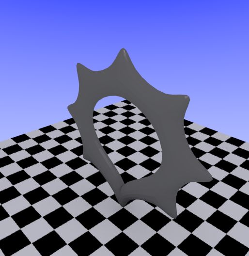
Technical University of Denmark
Informatics and Mathematical Modelling
Building 321, DK-2800 Kongens Lyngby, Denmark
Phone +45 45253351, Fax +45 45882673
reception@imm.dtu.dk
www.imm.dtu.dk
Summary

The costs of developing blockbuster video games are growing fast with a large
part spent on artists creating 3D models. New procedural modeling techniques,
such as the Skeleton to Quad-dominant Mesh (SQM) method by Bærentzen
et al. [15], could potentially reduce the costs of creating 3D models. The SQM
method is skeleton based, and allows the artist to create 3D models from a tree
with nodes.

The thesis explores the limits of SQM and the Skeleton Modeler by setting
modeling goals and trying to model them. The SQM method and associated
Skeleton Modeler is shown to be unfit for modeling non-organic shapes and
concavities.

The SQM method and Skeleton modeler is improved by extending the skeleton
with seven new nodes types. The new node types will not change the SQM
mesh generation, but extend it through pre- and post-processing steps.

The results show that the new node types enabled new shapes, but did not
improve the modeling goals. The results also show that concavities are not
easily representable in a skeleton based system.

The results for non-organic shapes can be improved by continuing with the se-
lected approach, but it is recommended to instead change the mesh generation
to simplify the algorithms. This will in turn require simplifications of SQM.
Concavities need a different approach, and integrating sculpting tools is a po-
tential solution that could to be explored.
ii

Preface

This master thesis was written as a part of the requirement for obtaining a degree
in Master of Science in Digital Media Engineering at the Technical University
of Denmark (DTU). The work was supervised by J. Andreas Bærentzen from
The Institute of Informatics and Mathematical Modelling at DTU.

                          Kongens Lyngby, February 2012

                          Michael Mc Donnell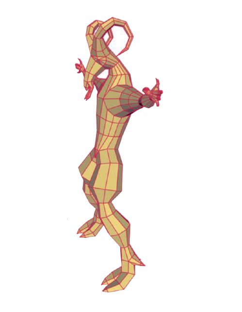
iv
Acknowledgements

I would like to thank my thesis supervisor J. Andreas Bærentzen. The thesis
is an attempt to expand the Skeleton to Quad-dominant Method (SQM) by
him and others [15]. The thesis topic and some of the proposed methods were
suggested by him.

I would finally like to thank my family and my Fiancé for supporting me and
cheering me on.
vi
Contents

Summary                                                                                                                          i

Preface                                                                                                                         iii

Acknowledgements                                                                                                                 v

1 Introduction                                                                                                                   1
  1.1 Motivation . . . . . . . . . . . . . . . . . . . . . . . . . . . . . .                                                     2
  1.2 Goals and Scope . . . . . . . . . . . . . . . . . . . . . . . . . . .                                                      3

2 Background Theory and Concepts                                                                                                 5
  2.1 Skeleton and Rooted Tree . . . . . . . . . . . . . . . . . . . . . .                                                       5
  2.2 Meshes . . . . . . . . . . . . . . . . . . . . . . . . . . . . . . . . .                                                   6
  2.3 Valency and Extraordinary Vertices . . . . . . . . . . . . . . . .                                                         6

3 SQM and the Skeleton Modeler                                                                                                   7

4 Goals and Limitations                                                                                                         11
  4.1 Modeling a Ladder . . .       .   .   .   .   .   .   .   .   .   .   .   .   .   .   .   .   .   .   .   .   .   .   .   13
  4.2 Modeling a Gear . . . .       .   .   .   .   .   .   .   .   .   .   .   .   .   .   .   .   .   .   .   .   .   .   .   16
  4.3 Modeling a Lollipop . .       .   .   .   .   .   .   .   .   .   .   .   .   .   .   .   .   .   .   .   .   .   .   .   20
  4.4 Modeling a Head . . . .       .   .   .   .   .   .   .   .   .   .   .   .   .   .   .   .   .   .   .   .   .   .   .   22
  4.5 Summary of Limitations        .   .   .   .   .   .   .   .   .   .   .   .   .   .   .   .   .   .   .   .   .   .   .   24

5 Improving SQM and The Skeleton Modeler                                                                                        25
  5.1 New Leaf Node Types . . . . . . . . . . . . .                                 .   .   .   .   .   .   .   .   .   .   .   25
  5.2 The Extended SQM Tree . . . . . . . . . . .                                   .   .   .   .   .   .   .   .   .   .   .   28
  5.3 Cube Node . . . . . . . . . . . . . . . . . . .                               .   .   .   .   .   .   .   .   .   .   .   29
  5.4 Root Branch Node Requirement . . . . . . .                                    .   .   .   .   .   .   .   .   .   .   .   29
viii                                                                                                                       CONTENTS

       5.5   Concavities . . . . . . . . . . . . . . . . . . . . . . . . . . . . . .                                                           30
       5.6   Cycles . . . . . . . . . . . . . . . . . . . . . . . . . . . . . . . . .                                                          31
       5.7   Remaining Limitations . . . . . . . . . . . . . . . . . . . . . . . .                                                             31

6 Hemisphere Node                                                                                                                              33
  6.1 Analysis . . . .         .   .   .   .   .   .   .   .   .   .   .   .   .   .   .   .   .   .   .   .   .   .   .   .   .   .   .   .   33
  6.2 Implementation           .   .   .   .   .   .   .   .   .   .   .   .   .   .   .   .   .   .   .   .   .   .   .   .   .   .   .   .   35
  6.3 Results . . . . .        .   .   .   .   .   .   .   .   .   .   .   .   .   .   .   .   .   .   .   .   .   .   .   .   .   .   .   .   36
  6.4 Sub-Conclusion           .   .   .   .   .   .   .   .   .   .   .   .   .   .   .   .   .   .   .   .   .   .   .   .   .   .   .   .   38

7 Cone Node                                                                                                                                    39
  7.1 Analysis . . . .         .   .   .   .   .   .   .   .   .   .   .   .   .   .   .   .   .   .   .   .   .   .   .   .   .   .   .   .   39
  7.2 Implementation           .   .   .   .   .   .   .   .   .   .   .   .   .   .   .   .   .   .   .   .   .   .   .   .   .   .   .   .   40
  7.3 Results . . . . .        .   .   .   .   .   .   .   .   .   .   .   .   .   .   .   .   .   .   .   .   .   .   .   .   .   .   .   .   40
  7.4 Sub-Conclusion           .   .   .   .   .   .   .   .   .   .   .   .   .   .   .   .   .   .   .   .   .   .   .   .   .   .   .   .   41

8 Leaf Sphere Node                                                                                                                             43
  8.1 Analysis . . . .         .   .   .   .   .   .   .   .   .   .   .   .   .   .   .   .   .   .   .   .   .   .   .   .   .   .   .   .   43
  8.2 Implementation           .   .   .   .   .   .   .   .   .   .   .   .   .   .   .   .   .   .   .   .   .   .   .   .   .   .   .   .   46
  8.3 Results . . . . .        .   .   .   .   .   .   .   .   .   .   .   .   .   .   .   .   .   .   .   .   .   .   .   .   .   .   .   .   46
  8.4 Sub-Conclusion           .   .   .   .   .   .   .   .   .   .   .   .   .   .   .   .   .   .   .   .   .   .   .   .   .   .   .   .   47

9 Negative Node                                                                                                                                49
  9.1 Analysis . . . .         .   .   .   .   .   .   .   .   .   .   .   .   .   .   .   .   .   .   .   .   .   .   .   .   .   .   .   .   49
  9.2 Implementation           .   .   .   .   .   .   .   .   .   .   .   .   .   .   .   .   .   .   .   .   .   .   .   .   .   .   .   .   50
  9.3 Results . . . . .        .   .   .   .   .   .   .   .   .   .   .   .   .   .   .   .   .   .   .   .   .   .   .   .   .   .   .   .   51
  9.4 Sub-Conclusion           .   .   .   .   .   .   .   .   .   .   .   .   .   .   .   .   .   .   .   .   .   .   .   .   .   .   .   .   52

10 Leaf Cube Node                                                                                                                              53
   10.1 Analysis . . . .       .   .   .   .   .   .   .   .   .   .   .   .   .   .   .   .   .   .   .   .   .   .   .   .   .   .   .   .   53
   10.2 Implementation         .   .   .   .   .   .   .   .   .   .   .   .   .   .   .   .   .   .   .   .   .   .   .   .   .   .   .   .   56
   10.3 Results . . . . .      .   .   .   .   .   .   .   .   .   .   .   .   .   .   .   .   .   .   .   .   .   .   .   .   .   .   .   .   57
   10.4 Sub-Conclusion         .   .   .   .   .   .   .   .   .   .   .   .   .   .   .   .   .   .   .   .   .   .   .   .   .   .   .   .   57

11 Connection Cube Node                                                                                                                        59
   11.1 Analysis . . . . . . . .               .   .   .   .   .   .   .   .   .   .   .   .   .   .   .   .   .   .   .   .   .   .   .   .   59
   11.2 Implementation . . . .                 .   .   .   .   .   .   .   .   .   .   .   .   .   .   .   .   .   .   .   .   .   .   .   .   60
   11.3 Results . . . . . . . . .              .   .   .   .   .   .   .   .   .   .   .   .   .   .   .   .   .   .   .   .   .   .   .   .   60
   11.4 Sub-Conclusion . . . .                 .   .   .   .   .   .   .   .   .   .   .   .   .   .   .   .   .   .   .   .   .   .   .   .   61

12 Branch Cube Node                                                                                                                            63
   12.1 Analysis . . . . .         .   .   .   .   .   .   .   .   .   .   .   .   .   .   .   .   .   .   .   .   .   .   .   .   .   .   .   63
   12.2 Implementation .           .   .   .   .   .   .   .   .   .   .   .   .   .   .   .   .   .   .   .   .   .   .   .   .   .   .   .   64
   12.3 Results . . . . . .        .   .   .   .   .   .   .   .   .   .   .   .   .   .   .   .   .   .   .   .   .   .   .   .   .   .   .   65
   12.4 Sub-Conclusion .           .   .   .   .   .   .   .   .   .   .   .   .   .   .   .   .   .   .   .   .   .   .   .   .   .   .   .   67
CONTENTS ix 13 Goals and Limitations Revisited 69 13.1 The Ladder Revisited . . . . . . . . . . . . . . . . . . . . . . . . 69 13.2 The Gear Revisited . . . . . . . . . . . . . . . . . . . . . . . . . . 70 13.3 The Head Revisited . . . . . . . . . . . . . . . . . . . . . . . . . 71 13.4 Interaction Between Nodes . . . . . . . . . . . . . . . . . . . . . 73 14 Conclusion 75 A Source Code 77 B User Guide 79 Bibliography 81
x CONTENTS
Chapter       1

                                               Introduction

The goal of the thesis is to improve the Skeleton to Quad-dominant Mesh (SQM)
algorithm presented in Bærentzen et al. [15]. The SQM Skeleton Modeler tool
uses lines to represent the bones in the skeleton and each bone is connected by
a sphere. The SQM algorithm is good for modeling objects that have a skeleton
structure, e.g. trees and base meshes for game characters. It, however, seems
to be limited to tapered branching objects. The work will be to analyze these
limitations and find solutions for them.

I will first present the motivation for why it is interesting to extend SQM,
and state the goals and scope of the thesis. Some of the background theory
necessary for understanding SQM will then be presented, and it can be skipped
and referred to later if needed. The SQM algorithm and the Skeleton will then be
described more in-depth before going into the meat of the thesis. Four modeling
goals are presented and modeled with SQM. These models reveal some of the
limitations of SQM, and ways around them are discussed in the subsequent
chapter. The discussion on the limitations in turn leads to the development of
seven new node types that are documented in-depth in their own chapters. The
new node types are then finally used to model the modeling goals again to see
if they have improved SQM.
2 Introduction 1.1 Motivation Over the last many years the cost of game development “skyrocketed”, according to Folmer [18], with console games costing on average between 3 and 10 million US dollars to develop. A large part of the cost is caused by the development time and team sizes, which have “nearly doubled over the last decade”. Folmer [18] focuses on how using commercial of the shelf (COTS) engines and tools can reduce the programming time and costs. One way that costs have already been brought down is by licensing game engines such as the Unreal Engine [8]. That way a game developer does not need to develop a whole engine, and the cost is shared among all the game developers licensing the engine. Licensing game engines is not the only way that costs have been brought down. There is also tools for generating content such as SpeedTree[7] for generating trees and foliage procedurally. Folmer [18] chose to focus on game engines and tools, but says that “the majority of the game development costs are spent on art and animation”. Another way to curb the cost is therefor to make the artists more efficient, which could be done through better animation and modeling tools. There are many modeling tools for helping the artist be more effective and pro- duce higher quality work. Some of these are dedicated sculpting tools such as Mudbox[4] and ZBrush[9], while others are more general tools such as Softimage[6] and Blender[1]. Most of these tools work directly with surfaces. SQM is dif- ferent because the artists specifies the surface implicitly by creating a skeleton connected by spheres and the SQM algorithm generates the surface from it. The artist can, therefore, quickly model the basic structure without worrying about the surface. One interesting property of using a skeleton structure is that it is suitable for integration with procedural generation such as L-systems [22]. Bærentzen et al. [15] showed that a tree could be procedurally generated and skinned with the SQM algorithm. Using procedural generation would relieve the artist from man- ually creating all the game content. He could instead generate a number of models by specifying a few parameters, and then choose the best result. Ji et al. [19] also generates meshes from a skeleton in their B-mesh method, and showed good results when using it to generate base meshes for game characters. The B-mesh tends to generate “three to four times more irregular vertices”[15, p. 8] than SQM, and SQM is therefore, a more interesting starting point for improving a skeleton based system. Leblanc et al. [20] uses blocks instead of spheres and is suitable for modeling non-organic shapes. It might be possible
1.2 Goals and Scope                                                               3

to combine the ideas and extend SQM to make it possible to create non-organic
shapes.

1.2     Goals and Scope

There are two goals for the thesis. The first is to document some of the limita-
tions of SQM. The second goal is to find simple methods to extend SQM with
new shapes.

The article by Bærentzen et al. [15] represents a large body of work, and it
is therefore out of the scope of the thesis to fundamentally change how SQM
works. The vertex and mesh generation is considered to be the fundamentals
of SQM, and the thesis will therefore focus on how it can be improved through
pre- and post-processing steps.

The scope of the implementation is to demonstrate the new methods for creating
shapes. The implementation is meant as a prototype and proof-of-concept, and
the focus will not be on code quality. It will need further work if it is to be used
in a production environment.

It is too early, and out of the scope of this thesis, to research if SQM is more
efficient than other modeling methods. There are no standardize methods for
comparing the efficiency of modeling techniques, and that is also out of a scope
of the thesis. I believe it is still important to develop new methods, as it is the
first step to become more efficient.
4 Introduction
Chapter       2
                Background Theory and
                            Concepts

This chapter contains an introduction to the background theory and concepts
necessary to understand the SQM algorithm. It can be skipped and referred to
later if needed.

2.1     Skeleton and Rooted Tree

SQM is a skeleton based method and uses a rooted tree to represent the skeleton.
The two terms will be used interchangeably throughout the thesis.

An informal introduction to rooted trees will now be given based on the defi-
nition in Cormen et al. [17, p. 1087] and Bærentzen et al. [15]. A rooted tree
consists of nodes that are connected by edges. The rooted tree starts in the root
node. The root node can be connected to other nodes via edges. The nodes that
are directly connected to the root node are called child nodes, and the root is
their parent node. Similarly the child nodes can have child nodes of their own,
to which they are their parent.

A node that does not have any children is called a leaf node. A node that has
6 Background Theory and Concepts exactly one child is called a connection node, and a node with more than one child is called a branch node. One important difference between a graph and a tree, is that a tree does not have any loops(also called cycles). That means it must not be possible to follow a path of edges in one direction and visit a node more than once. 2.2 Meshes A mesh is a graph that consists of vertices connected by edges. The vertices and edges form polygons. These polygons are typically triangles or quadrilaterals. A mesh consisting of triangles is called a triangle mesh, and a mesh the consisting of quadrilaterals is called a quad mesh. A quad-dominant mesh is a mesh that primarily consists of quadrilaterals and has few extraordinary vertices. SQM produces meshes that are quad-dominant. 2.3 Valency and Extraordinary Vertices The valency is the term for describing the number of neighbors a vertex has. In a triangle mesh a regular vertex has the valency of six [23]. Vertices in a triangle mesh that do not have a valency of six are called extraordinary vertices. The valency of a regular vertex in a quad mesh is four, and the extraordinary vertices in a quad mesh are those who do not have a valency of four.
Chapter       3
                   SQM and the Skeleton
                               Modeler

The Skeleton to Quad-dominant Mesh (SQM) method by Bærentzen et al. [15]
is an algorithm for generating a skin from a skeleton. The SQM article has
not been published at the time of the writing, so the description here will build
on the draft and source code from July 12th 2011, which can be found on the
accompanying CD-ROM or Zip-file. The SQM method has been improved in
the meantime, and has been accepted for the Shape Modeling International 2012
conference, so there will be some discrepancy between the final SQM description
and the one given here.

The skeleton in SQM is represented by a rooted tree. Each node in the tree
has a position and a radius, and a mesh is generated from the tree as seen on
Figure 3.1. The input skeleton for the SQM algorithm can be generated using
an interactive modeling tool, like the Skeleton Modeler written for SQM, or by a
program using a procedural approach like L-systems [22]. The Skeleton Modeler
represents the skeleton as a number of spheres connected by lines. The spheres
represent the nodes and their size and position can be manipulated by the user.

A quick overview of how the mesh is generated will now be given. The SQM
algorithm creates a branch node polyhedron (BNP) at each branch node and
connects them with tubes consisting of quads. If the node is a leaf node, then
the end of the tube is collapsed into a triangle fan. The radius of the node
8 SQM and the Skeleton Modeler
(a) Input skeleton (b) Generated mesh
Figure 3.1: The Skeleton Modeler in action. The skeleton is seen on the left and
the generated mesh on the right.
controls the size of the BNPs.
A more thorough description of the mesh generation will now be given. There
are are six steps in the SQM algorithm :
1. BNP generation
2. BNP refinement
3. Bridging
4. Final vertex placement
The BNP generation works by first finding the vertices by intersecting the edges
coming into the branch node with its associated sphere. Each BNP is then cre-
ated by performing a spherical Delaunay triangulation on each of these sets of
vertices. The SQM algorithm greedily refines the BNPs until they can be con-
nected by a tube of quadrilaterals. The BNPs are then bridged to form a single
mesh. The final vertex placement improves the look of the mesh by running
multiple iterations of Laplacian smoothing and finding an optimal position on
a tube using a quadric error measure.9 The SQM is interesting because of the quality of the mesh it generates. The SQM algorithm produces a quad-dominant mesh with extraordinary vertices in the joints (BNPs) and at the tips. SQM generates fewer extraordinary vertices compared to the B-Mesh method by Ji et al. [19]. The quads tend to be aligned in the direction of the curvature lines, which is similar to what an artist would do [14]. The tips are where the tubes were collapsed. The tips form polar regions, which means that they are triangle fans surrounded by quads. This makes the mesh suitable for Bi-3 C 2 polar subdivision (C 2 PS) by Myles and Peters [21]. If the mesh is subdivided with C 2 PS, then it will not develop unwanted creases in the tips, as would otherwise be the case if the more popular Catmull-Clark subdivision [16] is used. The Skeleton Modeler has a subdivision implementation that can handle polar regions, but it is not a full implementation of C 2 PS.
10 SQM and the Skeleton Modeler
Chapter 4
Goals and Limitations
A good way to analyze the limitations of the SQM algorithm and the Skeleton
Modeler is to set a goal for modeling various objects, and try to see if the goal
is possible to model. In [15] several objects were modeled to understand the
performance and limitations of the SQM method. Some of these objects can be
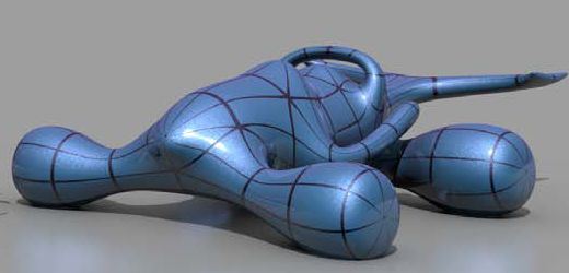
seen on Figure 4.1 (a-c) on page 12. The goat creature on Figure 4.1a and the
tree on Figure 4.1b are both organic objects, and they look fairly convincing.
The car on Figure 4.1c, which is a non-organic object, however, looks too organic
to be convincing. This suggests that SQM or the Skeleton Modeler might be
less than ideal for modeling non-organic objects.
It is not clear which part of the SQM that makes it difficult to produce non-
organic looking objects. It could very well be that the SQM is suitable for
modeling non-organic objects, and it is just the associated Skeleton Modeler
tool that makes it difficult to produce the correct input for the SQM algorithm.
In this chapter the limitations of SQM and the Skeleton Modeler will be analyzed
through modeling goals. The first goals are a ladder and a gear. They were
chosen because they are more simple than a car but still complicated enough
to reveal some of the limitations. A lollipop will also be modeled to see if it is
possible to create spherical shapes. This will also serve as a starting point for
modeling a head. The head was chosen because it contains concavities.12 Goals and Limitations
(a) A goat creature (b) A tree
(c) A car
Figure 4.1: Examples of some of the objects modeled by Bærentzen et al. [15]
with SQM.4.1 Modeling a Ladder 13
4.1 Modeling a Ladder
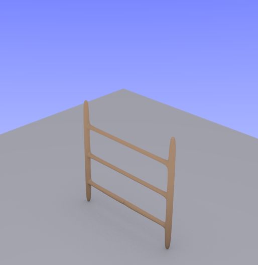
A simple ladder, as seen on Figure 4.2, was chosen as a modeling goal. It was
modeled using Blender[1], which is a traditional 3D content creation suite. The
ladder was chosen because it is symmetric, it consists of rectangular and round
shapes, and it has loops. It consists of two elongated boxes connected by three
tubes that are slightly offset in relation to the boxes edges. The ladder is clearly
symmetric around a vertical center line. It can also been seen that the ladder
could be cut into three identical parts using two horizontal planes.
Figure 4.2: A simple ladder created with Blender.
The Skeleton Modeler starts with a red root node in the middle of the screen in
symmetric mode. Figure 4.3 shows the Skeleton Modeler started up and rotated
slightly around the red root node to reveal the default vertical green symmetry
plane. Any nodes that are added to the root node will be mirrored around the
symmetry plane. It, therefore, seems obvious to crate one of the round tubes
by going through the root node as seen on Figure 4.4a on page 14. This simple
shape reveals the first limitations: The Skeleton Modeler cannot skin the bone
structure and outputs the error message “Root must be a branch node!”.
Figure 4.3: The root
node and the symme-
try plane.
It is possible to work around the limitation that the root node must be a branch
node by placing a node in the exact same position as the root node, as seen on
Figure 4.4b. This is, however, difficult because there is no automatic snapping14 Goals and Limitations
(a) No branching (b) Branch on root (c) Skinned
(d) Consolidated (e) Skinned (f) Subdivided
Figure 4.4: Creating a straight tube with Skeleton Modeler.
and the node has to be placed in the exact same position as the root node. It
is also difficult to move the node afterwards without selecting the root node.
After the straight piece has been created it can be skinned by pressing the
space bar. The result can be seen on Figure 4.4c. The resulting model does not
look like a tube because it is pointy instead of flat in both ends. The Skeleton
Modeler has a feature called “consolidate leaves” that can make the leaves less
pointy by placing an extra node at a small distance from all the nodes in their
respective directions. The distance is dependent on radius of the spheres in the
leaf nodes. It can be activated by pressing shift-c and the result can be seen on
Figure 4.4d. Please note that the new node on top of the node on the root node
has been deleted with the x key. Skinning the skeleton with consolidated leaves
produces the result seen on Figure 4.4e. The ends are still not flat but they can
be made more flat by manually moving the new nodes closer to the original leaf
nodes. It is, however, again like in the case of the root node, difficult to move
the nodes directly on top of leaf nodes. Creating flat ends is, therefore, clearly
another limitation that needs to be addressed.
The tube with pointy ends on Figure 4.4e looks similar to two boxes next to
each other, rotated 90◦ , and with pyramids on the ends. When it is subdivided
it looks close similar to a tube, except for the round ends, as seen on Figure 4.4f.
This result should be good enough for creating the tube sections in the ladder,
but there is no way to explicitly create boxes, which is another limitation that
needs to be solved.
With the current limitations in mind we will now try to create a ladder. The
skeleton structure is first created as seen on Figure 4.5a. It is then skinned
which results in the mesh seen on Figure 4.5b. The mirror symmetric leaf nodes
close to each other can be merged after the skinning process by pressing the m
key. The Skeleton Modeler does this by modifying mesh. It removes the vertices
corresponding to close mirror leaf nodes and bridges the one rings. The result
of merging the close leaf nodes can be seen on Figure 4.5c. There is no way to
specify how close the leaf nodes need to be, so it could potentially merged some4.1 Modeling a Ladder 15
(a) The skeleton (b) Unmerged
(c) Merged (d) subdivided
Figure 4.5: A ladder created with the Skeleton Modeler.
(a) The skeleton (b) Merged (c) Subdivided
Figure 4.6: The ladder with sharper joints.
wrong leaf nodes. This is another limitation. It would be helpful to be able to
either model loops, or specify which nodes need to be merged.
The ladder was then subdivided as seen on Figure 4.5d. The parts that were
supposed to be boxes are rounded as seen before when creating the straight
piece. This is the same limitations as noted before. It is not possible to specify
hard edges nor control the rotation. It can also be seen that joint where the tube
parts meet the boxes is rounded instead of creating sharp 90◦ angled joints. The
joints can be made sharper by using a workaround similar to the consolidate
leaves one. If an extra node is placed in the joint, then the joint is forced to be
sharper as can be seen on Figure 4.6. They are, however, still not completely
sharp, so this is another limitation.
Another detail that was left out from the modeling the ladder on Figure 4.616 Goals and Limitations
(a) The skeleton (b) Merged (c) Subdivided
Figure 4.7: The ladder with offset and smaller tubular steps.
(a) Goal (b) Result
Figure 4.8: A comparison of the goal created with Blender and the result created
with the Skeleton Modeler.
was that the tubular steps connecting the boxes were slightly offset from the
edge, and that they are smaller than the boxes. There is no way to specify this
explicitly, but it can be done by scaling down the size of the spheres inserted
for creating the sharper joints. The result of this can be seen on Figure 4.7.
The final result is compared to the goal on Figure 4.8. The ladder created with
the Skeleton Modeler looks somewhat similar to the goal on, if we ignore the
exact dimensions and the thickness of the parts. The biggest difference is that
the boxes on the side have been rounded, the tops ends are round, the joints are
not 90◦ angles, and there is a glitch in the middle of the bottom step. There is,
therefore, an opportunity to improve SQM to better handle theses cases.
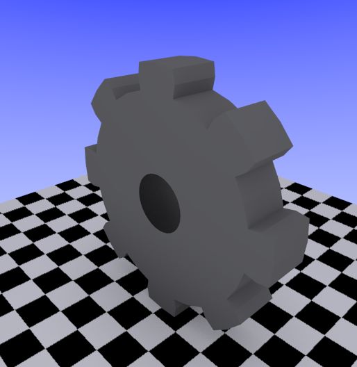
4.2 Modeling a Gear
In this section the goal is to create a simple gear with the Skeleton Modeler.
The goal seen on Figure 4.9 was created procedurally with Blender’s “Extra
Objects” plug-in. The gear can be composed into simpler objects like in the
case of the ladder. The main part is a tube with thick walls, and it has eight4.2 Modeling a Gear 17
teeth around its side each separated by 45 degrees angles.
Figure 4.9: A simple gear created with Blender.
There is no way to directly create a tube with thick walls, so one approach
would be to create a ring structure as seen on Figure 4.10a with eight spokes.
Placing the spokes and creating 45 degree angles had to be done manually, but
the skeleton modeler could be extended to help with the placement. Aside for
the non-perfect node placement, the bottom part of the ring looks odd when
skinned as seen on Figure 4.10b. This is because the nodes at the bottom have
not been merged. The SQM algorithm does not support cycles as mentioned
earlier in the previous section, but the modeler can merge the mesh if two leaf
nodes are close to the symmetry plane. The two bottom nodes in the ring are,
however, not leaf nodes, so they are not merged. The bottom spoke on the other
hand is a leaf node, which is why the merged mesh on Figure 4.10c looks odd.
It could in principal be worked around by placing a pair of leaf nodes on top of
the nodes in the bottom of the ring, but it would be difficult to place the nodes
precisely. It can, therefore, be seen as earlier, that it is a limitation that cycles
cannot be expressed explicitly.
On Figure 4.10 it can also be seen that the hole in the middle of the ring is much
larger than the reference on Figure 4.9. The spheres in the ring can be made
larger, which makes the walls of the tube thicker as seen on Figure 4.11, but
it also makes the tube thicker in the other direction. It can, therefore, be seen
that it is not possible to independently control the width and height of nodes.
The final result can be seen next to the goal on Figure 4.12. It can be seen that
the gear becomes rounded when subdivided, whereas a flat tube was the goal.
Another limitation is, therefore, that it is not possible to make big flat sides on
non-leaf nodes. It can also be seen that the teeth are not box shaped and the
corners have been rounded. This is the same limitation with sharp angles and
box shapes that was seen when modeling the ladder.18 Goals and Limitations
(a) Gear ring (b) Odd bottom (c) Odd merge
Figure 4.10: An attempt to create a gear with the skeleton modeler.
(a) Thicker ring (b) Skinned
(c) Skinned side view (d) Original side view
Figure 4.11: Making the spheres in the ring larger makes the wall of the tube
thicker in both directions.4.2 Modeling a Gear 19
(a) Goal (b) Result
Figure 4.12: The final result compared with the goal.20 Goals and Limitations
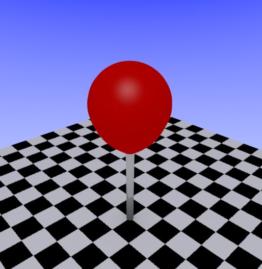
4.3 Modeling a Lollipop
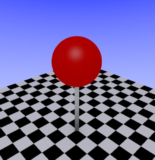
In this section the goal is to create a lollipop in order to find out if it is possible to
create spherical shapes. The goal seen on Figure 4.13 was created with Blender.
It consists of a sphere on top of a cylinder with closed ends.
Figure 4.13: A lollipop created with Blender.
Creating a sphere with the Skeleton Modeler requires more than just placing a
node. For example, the root node must be a branch node as seen earlier. The
SQM algorithm tries to create branch like structures, which means that in order
for the joint to become round, there must be branches in all directions. This
means that six nodes are needed as seen on Figure 4.14. The joint between
the sphere and the cylinder was made sharper by inserting an extra node right
under the root node, and finally the bottom of the cylinder was made more flat
by inserting an extra node at the bottom.
The final result was textured and rendered in Blender and is compared with the
goal on Figure 4.15. The result and goal look similar, and the biggest difference
is that the sphere in the result is not completely round but slightly elongated
at the bottom.4.3 Modeling a Lollipop 21
(a) Skeleton (b) Skinned (c) Subdivided
Figure 4.14: A lollipop modeled with the Skeleton Modeler.
(a) Goal (b) Result
Figure 4.15: The result compared with the goal.22 Goals and Limitations
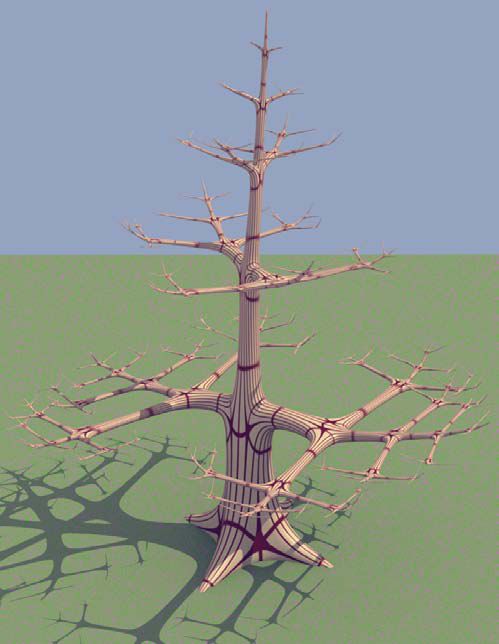
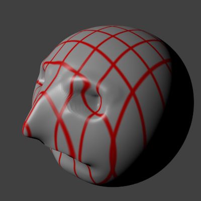
4.4 Modeling a Head
In this section the goal is to create a simple head model in order to uncover
potential limitations of SQM and the Skeleton Modeler. The goal seen on Fig-
ure 4.16 was modeled using Blender. A subdivided cube was used as the base
mesh, and the features were added by moving the vertices using the grab sculpt-
ing tool. The main features are the eye sockets, nose and mouth. The eye sockets
are almost ellipsoid concavities, whereas the mouth curves down at the sides.
Figure 4.16: A simple head modeled with Blender.
Figure 4.17 shows the result of creating a simple head with the Skeleton Modeler
and SQM. The round shape was accomplished in the same way as for the lollipop
in Section 4.3, by placing nodes on all sides of the root node, and then scaling
the root node up in size until it encompasses the nodes. The concavities for the
eye sockets and the mouth were created by placing nodes under the surface of
the root node, which forces the mesh back in.
(a) Initial skeleton. (b) Root node scaled (c) Skinned.
up.
Figure 4.17: The result of creating a simple head with the Skeleton Modeler.4.4 Modeling a Head 23 The biggest limitation that was discovered was that it is difficult to create concavities. The nodes used for creating the concavities have to be placed inside other nodes. That makes it difficult to see what the result of the input tree will be. It also makes it difficult to manipulate the concavities, as the node that encompasses it will have to be scaled down or moved before the node used for the concavity can be moved. It is also not possible to control the shape of the concavity. The mouth for example was supposed to be an elongated concavity, but it can be seen that there is a tube sticking out of the mouth. This is because three nodes were used to create the concavity and the SQM tries to build a mesh that follows that tree structure. There is also no way to express concavities in relation to the generated mesh.
24                                                          Goals and Limitations

4.5       Summary of Limitations

The following limitations were found in this chapter:

     • The root node must be a branch node.

     • Difficult to produce flat end pieces.
     • Not possible to create boxes.
     • Not possible to mark sharp edges for the subdivision.

     • Not possible to create sharp joints.
     • Difficult to place nodes according to a pattern, e.g. 45 degree angles.
     • Cycles cannot be expressed explicitly.
     • Not possible to control node width and height independently.

     • Not possible to make flat parts in non-leaf nodes.
     • Difficult to create spheres.

The next chapter discusses how to improve SQM and the Skeleton Modeler to
remove the limitations.
Chapter 5
Improving SQM and The
Skeleton Modeler
In this chapter we will look into how SQM could be extended to handle more
shapes. The chapter is meant as an overview and the details of the implemen-
tation and results will be described in later chapters.
5.1 New Leaf Node Types
In the previous chapter it was seen that it was difficult to produce flat end pieces.
The SQM algorithm connects the two nodes with a cylinder but collapses leaf
nodes to a point which result in a cone as seen on the simplified 2D illustration
on Figure 5.1. The figure shows a section of the SQM tree with a connection
node and a leaf node. The solid line represents the bone and the stippled line
represents the generated mesh.
One way to solve the problem with the flat end pieces could be to add a special
leaf node that is flat, e.g. a hemisphere leaf node. There is, however, no reason
to stop at flat end pieces. One could also think other types of end pieces that
could expressed with new leaf node types. Four proposed leaf node types can
be seen on Figure 5.2 on page 27 drawn in a light gray. The four proposed leaf26 Improving SQM and The Skeleton Modeler
node types are:
• Hemisphere leaf nodes
• Sphere leaf nodes
• Cone leaf nodes
• Cube leaf nodes
Common for the proposed leaf node types is that they do not change the basic
mesh properties. The leaf nodes are still polar regions. We will now go through
the four new node types.
Sphere node
Bone
Sphere node
Figure 5.1: The current behavior of a leaf node.
The hemisphere node would allow the creation closed cylinders. The hemisphere
leaf node is represented by a closed hemisphere. It is rotated so that the normal
of the flat side points in the direction of the bone and away from the center of
the parent. The two nodes should be connected by a cylinder with a flat closed
end or a truncated cone.
The new leaf sphere node changes the behavior so that the end is round instead
of pointy. This makes the generated mesh correspond more closely to the input
skeleton. The representation of the new leaf sphere node looks just like the old
sphere node, but the nodes will be connected by a cylinder or truncated cone
with a hemisphere on the top.
The cone node provides a way to explicitly make ends pointy. The cone node
should behave in the same way as the old leaf sphere node on Figure 5.1. The
representation should be a cone which changes its size and direction automati-
cally when the user moves the tip of the cone. The bottom of the cone should5.1 New Leaf Node Types 27
Hemisphere node Sphere node Cone node Cube node
Bone Bone Bone
Bone
Sphere node Sphere node Sphere node Sphere node
(a) (b) (c) (d)
Figure 5.2: The four proposed node types.
go through the center of the parent node, and the normal of the bottom side
should be aligned with the bone and point towards the center of the parent.
The bone ends in the tip of the cone.
The cube leaf node would enable box shapes. It is represented by a cube that
can be scaled in all directions. It can also be rotated around the bone axis,
which means the bottom normal should point towards the center of the parent
node. The SQM algorithm should be modified so that the bottom of the cube is
connected with the sphere using a tubular shape consisting of quads. One end
of the tube should approximates a circle end other end should approximate a
rectangle shape. The cube is subdivided until it is possible to connect the two
kinds of shapes. Finally the top should be triangle fan so that the part of the
mesh resulting from the leaf node remains a polar region.
All of these nodes should be possible to implement using a tree transform, which
is explained in the next section.28 Improving SQM and The Skeleton Modeler
5.2 The Extended SQM Tree
A number of new node types were suggested in the previous section in this
chapter. One way to implement these new node types is to modify the SQM
algorithm to directly generate the new shapes that the new node types represent.
Another way would be to create an Extended SQM tree (ESQM tree). The
ESQM tree would contain the new nodes types and would be converted into the
old SQM tree before the SQM algorithm is run. That way the SQM algorithm
itself would not need to be changed.
In the section where a ladder was modeled, it was seen that the leaf nodes could
be more flat by using the “consolidate leaves” operation on the leaf nodes. This
was done by inserting extra nodes close to the leaf nodes as seen on Figure 4.4d
on page 14. One could imagine that the end would become completely flat if
new extra node is placed directly on top of its parent instead of close to it. It is,
however, difficult to place them on top of each other with a mouse. Furthermore,
it is cumbersome to move the nodes together manually, if the position of the
original node needs to be edited.
The leaf hemisphere node could be implemented using the ESQM tree approach.
It would then be implemented by converting it to a node with a an extra node
on top of it similar to how “consolidate leaves” operation worked. The user
would only see and move the new hemisphere leaf node type, thus the problem
with the exact placement and editing would be solved.
ESQM tree transfor-
mation to SQM tree
Figure 5.3: Transforming the new leaf sphere node in the ESQM tree into
multiple nodes in the SQM tree.
The new leaf sphere node type could also be implemented using the ESQM
approach. Instead of just adding an extra node as in the case of the leaf hemi-
sphere node, multiple nodes could be used to approximate a sphere as seen on5.3 Cube Node 29 Figure 5.3. The subdivision depends on the number of nodes, and the level of subdivision could be made user controllable. 5.3 Cube Node New leaf node types were defined in the previous sections. The idea could be expanded to also include new non-leaf node types. A new cube node could for example make it possible to create cube shapes, e.g. for creating a ladder. Like the leaf cube node, the non-leaf cube could be scaled in any direction, and rotated along the bone axis. One way to implement cube nodes could be to modify the final vertex placement step. The vertices could be moved out into corners of the cube and the remaining vertices could be distributed on the edges. This would not require changes to SQM but could be applied as a post-process. 5.4 Root Branch Node Requirement The SQM algorithm could be modified so that it does not require the root node to be a branch node. The BNP creation would have to change because the root node must have at least three children in order to create a BNP. Remember that this requirement comes from when the intersection between the root node’s sphere and the paths are performed. This results in two opposite triangles when it is has three children. It would produce two line segments if there are two children, and two points if there is one child. This would then cause a problem in the subsequent subdivision because there would not be any triangles to subdivide. One way to get around the subsequent subdivision problem is to make sure that triangles are created even with fewer than three connected nodes. If there are two children, then the orthogonal direction to the directions of the paths could be used to create a pseudo path. The intersection could then be performed between the node’s sphere and the pseudo path to create the missing points. Two pseudo paths could similarly be created if the root node only has a single child. Finally if the root has no children, then a sphere mesh could be created during the BNP creation and the remaining SQM steps could be skipped. This would not really be helpful in the number of new shapes it enables(only one), but it would be helpful in giving the artist some more logical feedback than an error message.
30                                Improving SQM and The Skeleton Modeler

The suggested method for removing the root branch node requirement will re-
quire changes to the BNP creation, which means that it is a fundamental change
to SQM. It is, therefore, considered out of the scope to implement this change.

5.5     Concavities

There is no way to explicitly specify a concavity in the Skeleton Modeler. It
seems to be a general problem with any bone editing system that there is no
obvious way to create concavities. For example, neither [19] nor [20] specify any
way to create concavities. Both add details in a post process using traditional
sculpting methods. The problem seems to be that in the real world there are no
objects that take away space. Putting flesh and skin on top of a bone structure,
however, corresponds well to how the real world works. Similarly sculpting and
carving is how an artist would remove material from an object. Sculpting tools,
therefore, seem like a natural way of creating concavities.

It is possible to create concavities with the SQM algorithm by moving a leaf
node back into its parent. It is, however, difficult to control. The first problem
is that the new leaf node is inside the node and therefore not possible to select
and manipulate with the mouse. The second, and probably most important
problem, is that there is no clear relationship between the position and size of
the leaf node, and the size and shape of the concavity. We will outline three
possible ways to improve the creation of concavities.

One way could be to add negative nodes leaf nodes. They would point out
of the parent, but would be moved back into the parent just before the SQM
algorithm is run. They would be easier to manipulate because they stick out of
the parent node. A negative node that is further away from its parent would
create a deeper concavity. Similarly a bigger negative node would create a wider
concavity. Negative leaf nodes could be implemented using an ESQM to SQM
tree transformation, which moves the negative node into the parent.

A second way could be to add a deformable node type. The deformable node
would have a mesh that could be deformed with traditional sculpting tools. The
SQM algorithm would have to be changed so that the final vertex placement
follows the deformation of the node. It is, however, not obvious how it would
affect the rest of the SQM algorithm, and how many changes would be needed.

Finally a third way to create concavities could be to display the generated mesh
and let the user manipulate it using sculpting tools. The sculpting operations
could then somehow be associated with nearby nodes and reapplied after the
5.6 Cycles                                                                     31

mesh is regenerated. That would make it possible to move and create nodes in
one part of the tree, while retaining details created in another part of the tree.
For example, a list of type, magnitude, relative position, and direction of the
sculpting operations could be stored in the closest node.

The first way would be easiest to implement as it would not require any changes
to the core of the SQM algorithm. It could be implemented as a simple trans-
formation of the input tree. The two last ways would require more work to
implement. The second way would require changes to the core of the SQM
algorithm, and it is not clear how much will need to be changed. The third
way could be done without changing the SQM algorithm, as it would be a post
process applied to the mesh after generating the mesh. The sculpting opera-
tions would be coupled to the tree, so the mesh could be regenerated without
discarding all the sculpting operations. The negative node will be implemented
as it requires the fewest changes.

5.6     Cycles

The SQM algorithm cannot handle cyclic graphs. It is possible to add cycles
using a built-in post-process. After the mesh generation the symmetric twin
leaf nodes that are close to each other are found. If they are closer than some
threshold then the parts of the meshes representing the nodes are bridged. This
means that it is not possible to explicitly control which nodes are merged.

A special cycle node could be added. The Skeleton Modeler would need to have
a way to select two nodes and mark them for merging. The artist would then
see a special node type in the Skeleton Editor. The merged node would be
broken into two separate nodes before the SQM algorithm is run and marked
for merging later. The SQM algorithm would be run to create the mesh, and
then finally the nodes marked for merging with each other would be merged.

Cycles have been chosen not to be implemented to limit the scope and will,
therefore, not be discussed further.

5.7     Remaining Limitations

Section 4.5 listed a number of limitations. All of them have not been addressed
in this chapter to limit the scope. They are, therefore, good choices for further
work.
32 Improving SQM and The Skeleton Modeler
Chapter       6

                                  Hemisphere Node

6.1      Analysis

During the modeling of a ladder in Chapter 4, it was seen that it was difficult to
produce flat end pieces. In Chapter 5 it was suggested that adding a hemisphere
node could make it easier to create rounded shapes such as cylinders with flat
tops and truncated cones. The hemisphere node illustration is repeated here on
Figure 6.1. The stippled line represents the generated mesh. The mesh between
the hemisphere node and the sphere node is a truncated cone or cylinder, where
the top radius matches the radius of the hemisphere node, and the bottom radius
matches the radius of the sphere node. The hemisphere node is represented by
a closed hemisphere. It should always be rotated so that the normal of the flat
side points in the direction of the bone and away from the center of the parent.
That way the flat end will be represented by the flat end of the filled hemisphere.

One straightforward way to implement the hemisphere node without changing
the SQM algorithm would be to use a tree transform as described in Section 5.2.
The hemisphere node in the ESQM tree would be replaced with two sphere nodes
in the SQM tree as seen on Figure 6.2. The SQM algorithm creates a single
vertex for the leaf node, so if the leaf node is in the same position as its parent’s
position, then a flat top with a polar region should be generated.
34 Hemisphere Node
Hemisphere node
Bone
Sphere node
Figure 6.1: A 2D illustration of the hemisphere node.
Hemisphere node
Bone Bone
Sphere node Sphere node
Figure 6.2: The hemisphere node in the ESQM tree is replaced by two sphere
nodes in the SQM tree.
Another approach to implementing the hemisphere node could be again to use
a tree transformation, but changing the positions of the new nodes. The hemi-
sphere node is again replaced by two sphere nodes as seen on Figure 6.3, but
the position of the leaf node is not directly on top of its parent. The position
of the leaf node is moved away in the direction of the bone. This is somewhat
similar to how the existing “consolidate leaves” feature works. The single vertex
resulting from the leaf node is then moved to the parent node’s position during
the final vertex placement.
The hemisphere node should also work with the subdivision scheme used in
Skeleton Modeler. The edges around the vertex created from the leaf node
would have to be marked in a special way. The subdivision scheme should be6.2 Implementation 35
Hemisphere node
Bone Bone
Sphere node Sphere node
Figure 6.3: An alternative way to implement the hemisphere. The hemisphere
node in the ESQM tree is again replaced by two sphere nodes in the SQM tree,
but the leaf node is not in the same position as its parent. The vertex in the
tip is moved down during the final vertex placement.
able to split the edges, but not move the original vertices. Furthermore, the
new vertices should remain in the same plane as the original vertices. This is
illustrated in 2D on Figure 6.4 where the mesh is subdivided once to better
approximate a disk. The mesh is illustrated with thick black lines, the stippled
circle is the limit surface, and the black dots are the vertices. It was decided
that modifying the subdivision implementation is out of the scope of the thesis,
so it will not be implemented.
Figure 6.4: An example of how the subdivision should progress to approximate
a disk.
6.2 Implementation
The tree transform as describe in the previous section was implemented. It
did however not work. The original SQM implementation by [15] cannot han-
dle nodes in the same position. In the method Graph::compute paths and -36 Hemisphere Node distances a 2D grid is initialized with the distances between the nodes. A non-calculated distance is represented by zero, so it is not possible to differenti- ate between the distance not being calculated and a distance of zero. The code was changed so that the grid was initialized with −1 instead of zero. That way a distance of zero could be stored in the grid. That was unfortunately not enough to make it work as there are also multiple places in the source code where the distance between a parent and a child node is used in a division (e.g. in the final vertex placement). This problem would require extensive changes to the original implementation, so it was chosen to instead try the second approach described in the previous section. This meant that the SQM tree had to be changed so that nodes resulting from the transformation had to be marked as hemisphere nodes. That way the vertex created by the leaf node could be identified and moved to the same position as its parent node during the final vertex placement. The visualization of the hemisphere node was implemented by modifying the source code of the freeglut project[10]. The code for visualizing a sphere was modified so that all the vertices belonging to the top half of the sphere would all be in the plane separating the top from the bottom half. This was done by setting the y coordinate to zero for all the vertices that had a positive y coordinate (y was the same direction as the up vector). The top of the hemisphere node should always be rotated, so that the normal points in the same direction as the bone. The rotation around the bone is not important as long as the mesh is not twisted with that rotation. The GEL library [2] contains the function make rot that can “Construct a Quaternion rotating from the direction given by the first argument to the direction given by the second.”. The direction of the bone and the default up vector is used as the input to construct the quaternion. The rotation axis and angle is then be found by using the get rot function in GEL. The rotation axis and angle is then supplied to glRotated in OpenGL [5] before drawing the hemisphere node. 6.3 Results A comparison of the straight piece created with the “consolidate leaves” feature and the hemisphere node can be seen on Figure 6.5. The end piece created with the hemisphere node is flat, whereas the one created with the “consolidate leaves” feature is pointy. That is a clear improvement in the quality of the shape. If the flat end needs to be moved, then the two nodes crated with the “consoli- date leaves” feature will have to be moved together, which can be cumbersome.
6.3 Results                                                                   37

The hemisphere is a single node, so it is no more difficult to move than a normal
node.

               (a) Consolidated               (b) Consolidated and skinned

              (c) Hemisphere node           (d) Hemisphere node and skinned

Figure 6.5: Comparison of a straight piece created with “consolidate leaves”
feature and the hemisphere node.

The results on Figure 6.5 shows a simple straight piece. The part of the mesh
resulting from each hemisphere node consists of only five vertices, four in the
circumference and one in the middle. That means that the flat end does not
approximate a disc very well. The number of vertices is dependent on the BNP
subdivision, and this can be forced higher by inserting more nodes. The result
on Figure 6.6 shows that the mesh in the top of the hemisphere node does indeed
approximate a disc when the BNP is more subdivided. Please not that the BNP
subdivision or refinement should not be confused with the subdivision scheme
that is included with the Skeleton Modeler and can be applied as a post-process.

       Figure 6.6: The top of the hemisphere node approximates a disc.

Figure 6.7 shows the straight piece created with hemisphere nodes and subdi-
vided using the subdivision scheme in the Skeleton Modeler. The straight piece
is not flat in the end. This is because hard edges were not implemented, nor
was the subdivision implementation improved to handle hard edges.
38 Hemisphere Node Figure 6.7: Straight piece created with hemisphere nodes and subdivided using the subdivision in the Skeleton Modeler. 6.4 Sub-Conclusion It was not possible to create flat ends with SQM. The Skeleton Modeler came with a feature called “consolidate leaves” that could insert extra nodes in order to create a more flat end, but it was still pointy. Another disadvantage of this feature was that two nodes would have to be moved together, if the artist wanted to move the flat end. It was assumed that a completely flat end could be created if the nodes were moved close enough together. This was discovered not to be true during the implementation phase. Here it was discovered that the current implementation assumed that the distance was non-zero, and that it became numerically unstable when the nodes were close together. The second approach therefore, had to be used where the nodes were placed at a distance, and the leaf node vertex moved during the final vertex placement. The hemisphere node solved the problem of having to use more than one node to create a flat end. A flat end is represented by a single node that can easily be moved. It was briefly outlined how the mesh generated from the hemisphere node could be subdivided. The subdivision implementation was, however, not changed because it was deemed out of the scope of the thesis. That meant that marking hard edges was also not implemented. This is something that could be looked into into as further work.
Chapter       7

                                                   Cone Node

7.1     Analysis

It was seen in Chapter 4 that using a leaf sphere node results in a single vertex
being created. This means that the resulting mesh, before being subdivided, is
shaped like a cone. It seems odd that the shape of the resulting mesh and the
shape of the node do not correspond to each other. A cone node could provide
a better connection between the input tree and the resulting shape.

The cone leaf node should behave in the same way as the old sphere leaf node
on Figure 5.1 and the SQM algorithm does, therefore, not need to be changed
for this node type. Figure 7.1 shows a simplified 2D illustration of how the
cone node should work. The representation should be a cone which changes its
size and direction automatically when the user moves the tip of the cone. The
bottom of the cone should go through the center of the parent node, and the
normal of the bottom side should be aligned with the bone and point towards
the center of the parent. The bone ends in the tip of the cone. Finally the
radius of the cone should be the same as the radius of the parent node.

The cone leaf node should also work with the subdivision scheme in the Skeleton
Modeler. None of the original vertices should be moved during the subdivision
and the new vertices should be placed in the same plane as the bottom plane
40 Cone Node
Cone node
Bone
Sphere node
Figure 7.1: The cone node illustration.
of the cone. This is the same way as the subdivision scheme described for the
hemisphere node in Chapter 6.
7.2 Implementation
The implementation was straightforward. The ESQM cone node is translated
to a single sphere node in the SQM tree.
The visualization of the cone node was implemented using the glutSolidCone
function in GLUT [3]. The distance between the cone node and the parent node
is used as the height, and the radius of the parent node is used as the radius of
the cone.
7.3 Results
The result of the implemented cone node can be seen on Figure 7.2. The gen-
erated mesh looks more like the input tree. The two results should have been
identical because the cone node is translated into an SQM sphere node. The
small difference is likely cause by the position of the extra node on top of the
root node. The extra node on top of the root node was added to work around
the requirement that the root must be a branch node.
One thing that was noticed, but cannot be shown on a figure, is that the cone7.4 Sub-Conclusion 41
node can become difficult to select when it is small or thin. This is because the
picking test is only done against the tip of the cone node out to the radius of the
resulting sphere node. The picking should be changed so that the whole cone is
used instead of just the tip.
(a) Old Input (b) Old result
(c) New input (d) New result
Figure 7.2: Comparison between the result of the old node sphere type and the
new cone node type.
7.4 Sub-Conclusion
The introduction of the cone node was motivated by the observation that there
was a poor correspondence between the shape of the sphere node and the result-
ing mesh. The resulting mesh was conical, so it was assumed that a cone node
would offer a better correspondence between the input tree and the resulting
mesh. The results confirmed this, but the usability has not been tested on any
artists.
The cone node in the current implementation can be difficult to manipulate
because only the tip of the cone node is used in the picking test. The pick-
ing should be changed so that the whole cone is used instead of just the tip.
Furthermore, the proposed changes to the subdivision implementation was not
implemented. These two extensions could be good candidates for further work.42 Cone Node
Chapter       8

                                Leaf Sphere Node

8.1     Analysis

The leaf sphere node in the original Skeleton Modeler resulted in a conical
shape. It seemed odd that a round node would result in a conical shape. The
cone node was therefore introduced in the previous chapter. It gave a direct
mapping between the input tree and the output mesh. In a similar way it could
be interesting to change the semantics of the sphere node, so that it results in
a spherical mesh instead of a cone.
44 Leaf Sphere Node
Sphere node
Bone
Sphere node
Figure 8.1: The new leaf sphere node.
Figure 8.1 shows a 2D illustration of how the new sphere node should work. Mul-
tiple vertices are inserted so that the mesh better approximates a hemisphere.
One way to implement this would be to use a tree transformation. Figure 8.2
shows how the new sphere node type in the ESQM tree could be translated
into multiple nodes in the SQM tree. Each SQM sphere node will result in a
edge ring being generated. The SQM sphere nodes radii decreases so that the
resulting mesh approximates a hemisphere.
ESQM tree transfor-
mation to SQM tree
Figure 8.2: The new leaf sphere node in the ESQM tree is translated into several
SQM sphere nodes.
Figure 8.3 shows how the radii of the generated sphere nodes could decay in
order to approximate a hemisphere. The left shows the 90 degrees arc that we
want to approximate, and the vertical lines represents the radii of the generated
sphere nodes in the SQM tree. The right shows a line segment connecting the
radii of the generated sphere node, and it can be seen that the line segmentsYou can also read