SKY DETECTION IN CSC-SEGMENTED COLOR IMAGES
←
→
Page content transcription
If your browser does not render page correctly, please read the page content below
SKY DETECTION IN CSC-SEGMENTED COLOR IMAGES

                                              Frank Schmitt, Lutz Priese
                                    University of Koblenz-Landau∗ , Koblenz, Germany
                                     fschmitt@uni-koblenz.de, priese@uni-koblenz.de

Keywords:      Sky detection, CSC

Abstract:      We present a novel algorithm for detection of sky areas in outdoor color images. In contrast to sky detectors
               in literature that detect only blue, cloudless sky we intend to detect all sorts of sky, i.e. blue, clouded and
               partially clouded sky. Our approach is based on the analysis of color, position, and shape properties of color
               homogeneous spatially connected regions detected by the CSC. An evaluation on a set of images acquired
               under different weather conditions proves the quality of the proposed system.

1     Introduction                                               2     Related and previous work

     For many applications in image processing accu-                 Previous work on sky detection by other groups
rate and fast detection of the sky is helpful. After the         has the goal to detect the pure blue sky, thus, the im-
sky has been detected we can conclude on the content             age of the atmosphere. Clouds are by this definition
of the image and extract information about weather               explicitly not part of the sky and therefore not to be
and illumination conditions during image acquisition.            detected.
Knowledge about the sky also often helps to constrain                Luo and Etz (Luo and Etz, 2002) state that the
the search domain for later, more complicated image              color of the sky changes gradually from a dark blue
recognition algorithms.                                          in the zenith to a bright, sometimes almost white, blue
     In images of urban regions the lower border of sky          near the horizon. They model the values in three color
areas often equals the top border of buildings. Those            channels along straight lines from zenith to horizon
borders can give first clues for pose estimation, i.e.           as three one-dimensional functions and analyze these
the detection of position and orientation of the cam-            functions with regard to characteristic properties of
era relative to the building. For this task it is important      the sky.
to find the sky reliable under all weather conditions,               Gallagher et. al (Gallagher et al., 2004) first gen-
i.e., cloudless, partially clouded or overclouded. On            erate an initial sky probability map based on classifi-
the other hand, it is not important to find smaller iso-         cation of color values. In a second stage they model
lated sky areas below such borders, e.g. under arch-             the spatial variation of pixels initially classified as
ways. The sky detection system introduced here is                sky. They calculate for each color channel a two-
optimized for such an application scenario.                      dimensional polynomial that approximates the values
     In the first steps of the algorithm, the input im-          of pixels with high sky probability. By comparison
age is smoothed and segmented by the CSC, a re-                  between values of pixels in the images and the corre-
gion growing segmentation method introduced by                   sponding values of the polynomial the final sky clas-
Rehrmann and Priese (Rehrmann and Priese, 1998).                 sification is generated.
The CSC partitions the image into spatially con-                     Zafarifar and de With (Zafarifar and de With,
nected, color homogeneous regions, called segments.              2006) use sky detection in the context of image qual-
Each segment is analyzed individually regarding its              ity enhancement in video data. Their system gen-
mean color and a sky probability is attached. In a fi-           erates a sky probability map based on texture, color
nal step spatial information typical for urban scenes            values, gradients, and vertical position in the image.
is added to the probability map and all segments are             They achieve very good results, however, they only
classified into sky and non-sky.                                 detect blue sky and therefore their system gives low
                                                                 sky probability in clouds.
    ∗ This
        work was supported by the DFG under grant                    However, in many parts of the world clouded sky
PR161/12-1 and PA 599/7-1                                        is very common. Thus, systems which restrict them-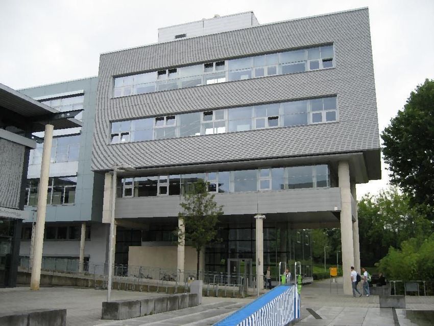
selves to blue sky detection are restricted in practica-        In a first step we smooth the image and segment it
bility. Our new system detects the total sky under all      into spatially connected, color homogeneous regions.
weather conditions.                                         In the next step we start at the top border of the image
    First ideas of the presented approach – not includ-     and search for segments whose mean color is suitable
ing the following major improvements based on the           for sky.
analysis of segment’s shape and gradients – have been           However, an analysis of mean color and position
presented in the German workshop “Farbworkshop              is insufficient. Such a straight forward method also
2008” (Schmitt and Priese, 2008).                           classifies white, gray, and blue objects outside the sky
                                                            - but immediately below the horizon - as sky. To re-
                                                            duce the number of those false-positive classifications
3    Characteristics of sky                                 we have to add another step where the shape of possi-
                                                            ble sky segments is analyzed.
    In systems for the detection of a cloudless sky one
may assume that the sky is free of large gradients but
shows a continuous brightness gradient. As we regard
                                                            4.2 Pre-processing and Segmentation
clouds as part of the sky we can not make such an
assumption. Our sky detector is thus based on differ-       The input image is first smoothed with one iteration of
ent assumptions and observations of characteristics of      a 3×3 Kuwahara-filter (M. Kuwahara, K. Hachimura,
the sky in color images in urban regions. We assume         S. Eiho, and M. Kinoshita, 1976). This non-linear
that the images to be analyzed have been acquired ho-       filter sharpens borders and simultaneously smooths
rizontally so that the sky is at the top of the image.      within homogeneous regions. The filtered image is
Where this assumption does not apply one may em-            segmented into spatially connected, color homoge-
ploy algorithms for horizon estimation as introduced        neous regions with the CSC.
in (Ettinger et al., 2002) or (Fefilatyev et al., 2006).
    Beside the position in the image, the color is the           The CSC is a region growing segmentation
second characteristic property of the sky. The color        method steered by a hierarchy of overlapping is-
can range from a pure white over different kinds of         lands. If two overlapping partial segments are simi-
gray inside clouds to shades of blue of different satu-     lar enough they are merged into a new segment. Else
ration and brightness in cloudless regions. We further      the common sub-region is split between them. As the
assume, that all segments belonging to the sky have a       decision whether to split or to merge two regions is
vertical connection to the upper border of the image,       not only based on a common border but a common
either directly or through other segments recognized        sub-region, the results are more stable than in con-
as sky.                                                     ventional region growing methods. The structure of
                                                            the island hierarchy makes the CSC inherently paral-
    If one chooses, e.g., split-and-merge (Horowitz
                                                            lel. Also, there is no need for spreading seed points
and Pavlidis, 1974) (SaM) as a segmentation tech-
                                                            in the image whose position influences the outcome
nique and the sky disintegrates into several seg-
                                                            of the segmentation in conventional region growing
ments the borders between those segments show large
                                                            methods.
straight lines. Those reflect the underlying quad-tree
structure of the SaM algorithm. This will not hap-               It is important to choose the parameters of the
pen with the CSC segmentation technique. The bor-           CSC such that an over-segmentation (areas belonging
ders of two segments of the sky almost always show          together are split into several segments) is more likely
an irregular contour without straight lines. However,       than an under-segmentation (areas not belonging to-
the border between sky and buildings is usually build       gether are merged into one segment) as an additional
from straight lines. This leads to further classification   classification of the found segments has to been done
criteria.                                                   anyway.
                                                                 The CSC segmentation can be applied either in
                                                            HSV color space based on color similarity tables
4    The algorithm                                          (Rehrmann, 1994) or in L*a*b* color space where
                                                            similarity between two shades of color is calculated
                                                            using the Euclidean distance. For the experiments in
4.1 Basic concepts                                          this paper we have chosen the L*a*b* color space
                                                            with a threshold of 12. The result of the CSC is a
Our algorithm is directly motivated by the observa-         label image where the value at every pixel is set to the
tions of the previous paragraph.                            label of the segment it belongs to.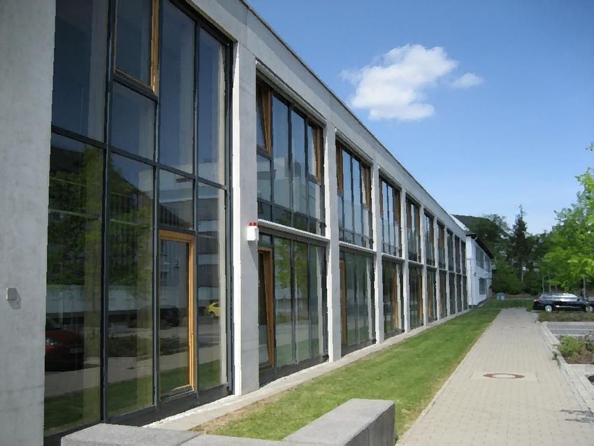
4.3 Characteristics of Segments                                4.4 Color analysis
Let a segment S be represented as a set of spatially           A classification of segments as sky solely by their
connected pixels. The upper border bu (S) consists of          color is obviously impossible. There are usually sev-
all coordinates (x, y) such that the pixel at (x, y) is in-    eral objects (or reflections) in an image that do not
side S and the pixel at (x, i) is outside S for all i ∈ N      belong to the sky but have a color which could also
with i < y. (As customary in computer vision, we use           occur in the sky. Thus, in this phase we only deter-
positive coordinates (x, y) where (0, 0) denotes the left      mine whether the mean color of a segment may occur
upper corner of the image.)                                    also in the sky. For such a task it will not help to
     The color of S is the mean color of all pixels be-        train a classifier with many examples of sky and non-
longing to S. As segments are color homogeneous,               sky segments. The result will not be disjunctive as all
the problem that averaging may create false colors             colors which can occur in the sky can occur in other
does not occur.                                                image regions as well. Instead, we were able to deter-
     The mean vertical gradient of S is a measure de-          mine by manual analysis of sample images a simple
scribing the brightness gradient at the common border          and rather compact subspace of the HSV color space
between S and its upper neighbor segments. It is cal-          which includes all colors occurring in sky.
culated as the average brightness difference between               Our experiments have shown that it suffices to call
pixels at bu (S) and their direct upper neighbor pixels.       a HSV value hsv sky colored if it meets at least one of
If no upper neighbors exist the mean vertical gradient         the following conditions:
is set to 0. A low mean vertical gradient is a strong            • hsv.saturation < 13 and hsv.value > 216
clue for a segment border generated during splitting             • hsv.saturation < 25 and hsv.value > 204 and
of a color gradient into several segments. Such bor-               hsv.hue > 190 and hsv.hue < 250
ders are normally more or less arbitrary and typical             • hsv.saturation < 128 and hsv.value > 153 and
for a segmentation within the sky.                                 hsv.hue > 200 and hsv.hue < 230
     The mean bounded second derivative of bu (S) is a           • hsv.value > 88 and hsv.hue > 210 and hsv.hue <
measure which describes whether the top border of S                220
is build of straight lines or rather formed irregularly.       The listed hue values are to some degree dependent
It is calculated as follows:                                   on the cameras used.
     Let xmin be the x-coordinate of the leftmost and
xmax of the rightmost pixel in S. For each i ∈ N               4.5 Analysis of position and shape
in [xmin , xmax ] exists exactly one coordinate with x-
component i in bu (S). We can therefore regard bu (S)          Let Ls and Lc be two (initially empty) lists of seg-
as a function of x where bu (S, x) := y if (x, y) ∈ bu (S)
                                                               ments already classified as sky (Ls ) or as candidates
and undefined else. The function
                                                               (Lc ) for sky. Segments whose mean color is sky col-
    δ2 (S, x) := bu (S, x − 1) − 2 · bu(S, x) + bu(S, x + 1)   ored and for which the condition holds that at least
                                                               half of their top border touches the top border of the
is the discrete second derivative of bu for segment S          image are added to Ls . All segments touching the
at position x.                                                 lower border of at least one of the segments in Ls are
    |δ2 (S, x)| is low at straight border segments and         added to a Lc . For each segment S in Lc we check
high at irregularly formed areas. Thus, an obvious ap-         three criteria:
proach would be to average |δ2 (S, x)| over the width
of S in order to get a measure for the straightness            1. the color of S is sky colored,
of S. However, this approach leads to the prob-                2. at least two thirds of the top border of S touches
lem that within a polygon, that consists of few con-              either the top border of the image or segments in
nected straight lines, the corner points may contribute           Ls ,
too high values. We therefore use bounded values               3. at least one of the following conditions is satisfied:
as follows: Let m(S, x) := 1 for |δ2 (S, x)| ≥ 1 and
m(S, x) := 0 elsewhere. The mean bounded second                  (a) the area of S contains less than 500 pixel (we
derivative of the top border of S is calculated as                   skip shape analysis for such small segments)
                                                                 (b) the mean vertical gradient of S is below 25
                          ∑          m(S, x)                     (c) the mean bounded second derivative of bu (S) is
                      (x,y)∈bu (S)
                                                                     bigger than 0.3.
                              ∑          1
                          (x,y)∈bu (S)                             If all three conditions are satisfied S is classified
.                                                              as sky and the lists Ls , Lc are updated. Otherwise, S is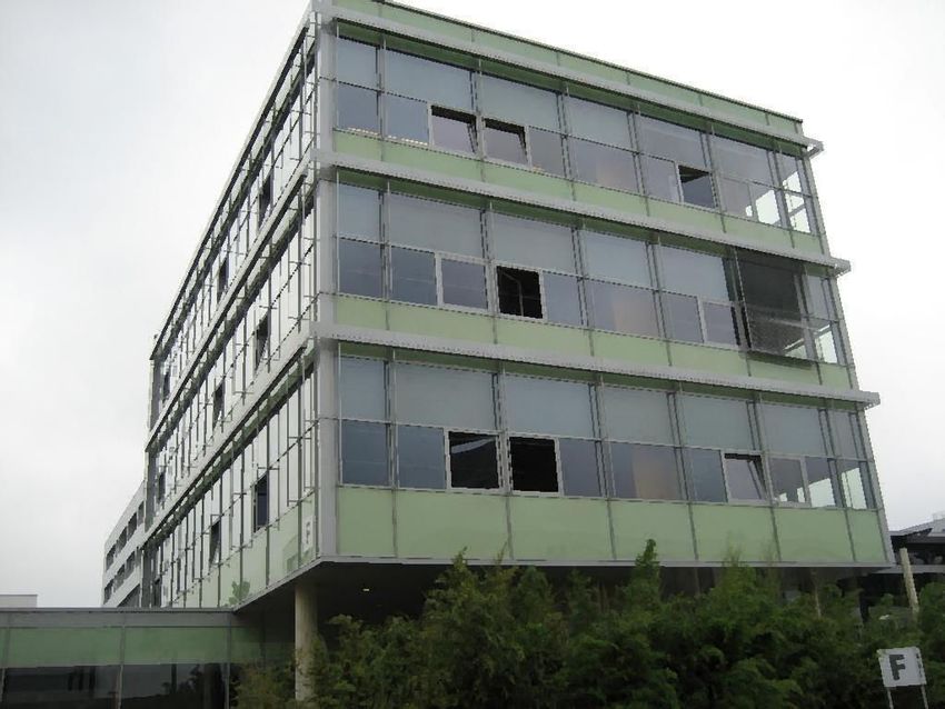
removed from Lc . The algorithm terminates when the
candidate list is empty.
    At this stage, all segments which belong to sky
and have a connection to the top border of the image
(either a direct connection or through other sky seg-      50
ments) should have been classified as sky. However,        40
in rare cases it may occur that, e.g., a cloud matches     30        Quantity
                                                           20
conditions 1 and 2 but not condition 3 and, thus, has      10
                                                                                                                                          1
                                                                                                                                    0.8
been falsely classified as non-sky. Such cases are de-      00                                                                0.6
tected and fixed in a post-processing step where all                  0.2
                                                                                0.4
                                                                                                                        0.4               CR
                                                                                        0.6                       0.2
non-sky segments which satisfy conditions 1 and 2                       ER                          0.8
                                                                                                            1 0
and which are completely surrounded by sky are clas-
sified as sky as well.

5     Evaluation                                                        Figure 1: Distribution of CR and ER

    For an evaluation 179 images of the campus of our
                                                           110
university have been acquired under different weather      105
                                                           100
conditions. Some examples are shown in appendix A.          95
                                                            90
                                                            85
To get a ground truth (GT) we have manually anno-           80
                                                            75
tated the sky to copies of those images. Our evalua-        70
                                                            65
                                                            60
tion compares the detected sky with this ground truth       55
                                                            50
sky with two measures: The coverability rate (CR)           45
                                                            40
                                                            35
measures how much of the true sky is detected by the        30
                                                            25
algorithm. The error rate (ER) measures how much            20
                                                            15
                                                            10
of the area detected as sky is not part of the true sky.     5
                                                             0
Let S denote the detected sky and GT the ground truth            0    0.1    0.2      0.3     0.4     0.5   0.6   0.7     0.8       0.9        1

sky. Then both measures are defined as
                                                                                Figure 2: Distribution of CR
                    |S ∩ GT |                 |S − GT |
    CR(S, GT ) :=             , ER(S, GT ) :=
                      |GT |                      |S|       125
                                                           120
                                                           115
                                                           110
                                                           105
    Graphic 1 visualizes our evaluation results. On        100
                                                            95
the x-axis the error rates are shown, on the y-axis the     90
                                                            85
                                                            80
coverability rates. The length of a line in z-direction     75
                                                            70
                                                            65
at position (x,y) tells in how many cases error rate x      60
                                                            55
                                                            50
and coverabiliy rate y was achieved. Graphics 2 and 3       45
                                                            40
                                                            35
show the distributions of CR and ER alone.                  30
                                                            25
                                                            20
    In 80% of all images, CR is above 0.9 and ER is         15
                                                            10
below 0.1. In 75% of all images, CR is above 0.95            5
                                                             0
                                                                 0    0.1    0.2      0.3     0.4     0.5   0.6   0.7     0.8       0.9        1
and ER is below 0.05. Those results clearly show the
quality of the proposed algorithm. The cases where                              Figure 3: Distribution of ER
the error rate is very high correspond in the majority
of cases to images that do not contain any sky at all.
As soon as our algorithm classifies at least one pixel
                                                           but also clouded sky. The presented algorithm is fast
as sky in those images the error rate becomes 1.0.
                                                           and an quantitative evaluation on a set of 179 images
                                                           shows its robustness.
                                                               We intend to further improve our sky detector and
6     Summary and Outlook                                  will try to automatically detect and split segments
                                                           which include both sky and non-sky, see Figure 7 as
    We have presented a fast and robust system for de-     an example. Also the detection of images in urban
tection of sky in camera images. In contrast to known      scenes without any sky at all could be improved.
systems, our algorithm is able to not only detect blue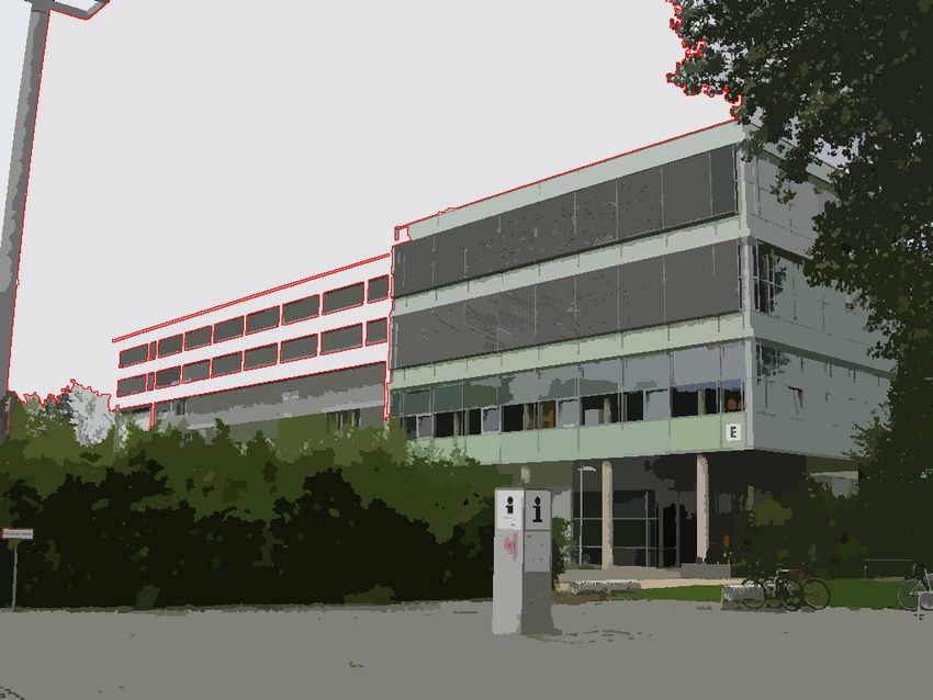
REFERENCES proach to detecting sky in photographicimages. IEEE
Transactions on Image Processing, 11(3):201–212.
Ettinger, S. M., Nechyba, M. C., Ifju, P. G., and Waszak, M. Kuwahara, K. Hachimura, S. Eiho, and M. Kinoshita
M. (2002). Towards flight autonomy: Vision-based (1976). Processing of ri-angiocardiographic images.
horizon detection for micro air vehicles. In Florida In Preston, K. and Onoe, M., editors, Digital Process-
Conference on Recent Advances in Robotics 2002. ing of Biomedical Images, pages 187–202.
Fefilatyev, S., Smarodzinava, V., Hall, L. O., and Gold- Rehrmann, V. (1994). Stabile, echtzeitfähige Farbbil-
gof, D. B. (2006). Horizon detection using machine dauswertung. PhD thesis, Universität Koblenz-
learning techniques. In ICMLA ’06: Proceedings of Landau, Fölbach Verlag, Koblenz.
the 5th International Conference on Machine Learn- Rehrmann, V. and Priese, L. (1998). Fast and robust seg-
ing and Applications, pages 17–21, Washington, DC, mentation of natural color scenes. In Chin, R. T.
USA. IEEE Computer Society. and Pong, T.-C., editors, 3rd Asian Conference on
Computer Vision (ACCV’98), number 1351 in LNCS,
Gallagher, A. C., Luo, J., and Hao, W. (2004). Improved pages 598–606. Springer Verlag.
blue sky detection using polynomial model fit. In Im-
age Processing, 2004. ICIP ’04. 2004 International Schmitt, F. and Priese, L. (2008). Himmelsdetektion in
Conference on, volume 4, pages 2367–2370. CSC-segmentierten Farbbildern. In Farbworkshop
2008, Aachen.
Horowitz, S. and Pavlidis, T. (1974). Picture segmentation
by a directed split-and-merge procedure. In Proceed- Zafarifar, B. and de With, P. H. N. (2006). Blue sky
ings of the Second International Joint Conference on detection for picture quality enhancement. In Ad-
Pattern Recognition, pages 424–433. vanced Concepts for Intelligent Vision Systems, vol-
ume 4179/2006 of Lecture Notes in Computer Sci-
Luo, J. and Etz, S. P. (2002). A physical model-based ap- ence, pages 522–532. Springer Berlin / Heidelberg.
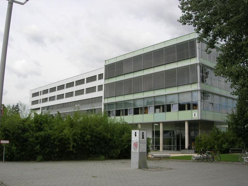
A Sample images
In the following images 4 to 6 the input image of our algorithm is shown on the left and the result of classifi-
cation on the right. White represents segments classified as sky, gray represents segments which are sky colored
but not classified as sky, black represents segments which are not sky colored.
Figure 4: Photo taken at sunshine with fair-weather cloudFigure 5: Photo taken in rainy weather
Figure 6: Sky colored segments in a building front which aren’t classified as sky due to shape analysis
The following picture 7 shows an example where the algorithm fails to correctly identify the sky. The segment
encircled in red was falsely classified as sky as even in the CSC-segmentation phase the white front was melted
into a larger sky segment.
Figure 7: Erroneous CSC segmentation: A white building front merges into one segment with the heavily clouded
skyYou can also read