Slow relaxation dynamics in the 2d spin-ice model
←
→
Page content transcription
If your browser does not render page correctly, please read the page content below
Slow relaxation dynamics in
   the 2d spin-ice model
        Demian Levis and Leticia Cugliandolo

    Laboratoire de Physique Théorique et Hautes Energies
                    Université de Paris VI

             Large Fluctuations in Non-Equilibrium Systems
                                     -
            Max Planck Institut für Physik Komplexer Systeme
                          Dresden, July 2011

                        arXiv: 1107.2528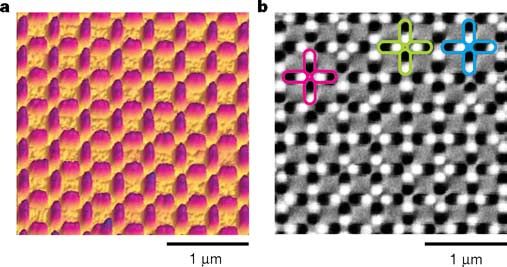
Slow relaxation dynamics in
   the 2d spin-ice model
  • Motivations.
  • Equilibrium properties.
  • Relaxation towards equilibrium.
  • Conclusions.

Motivations.

    Geometrical frustration

 Crucial example: water ice

   Experimental evidence of a finite entropy at T=0
              (Giauque & Stout 1936)
                                                                       ⇐=        Predicted by Pauling’s model (1935):

                                                                               at each vertex (oxygen atoms)
 ≡   each O-H bond carries a dipolar moment   � verifiying the ice-rules
                                              µ                            =    two dipoles point in and two out

                  � µ
 Ground state : { ∇.�      = 0 } Ice-rule vertices are favoured ⇒                   Geometrically frustrated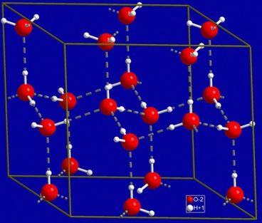
Motivations.

    Geometrical frustration
Crucial example: water ice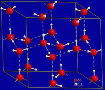
Motivations.

    Geometrical frustration
Crucial example: water ice                                                                   spin ice
                                                  Zero-point entropy on the pyrochlore lattice

                                                      �   Pyrochlore lattice = corner-sharing tetrahedra
                                                                         �        �2
                                                                   J� �
                                                          Hpyro =              σi
                                                                   2 tet
                                                                                  i∈tet

                                                      �   Pauling estimate of ground state
                                                          entropy S0 = ln Ngs :
                                                                        �        �N/2
                                                                    N       6              N 3
                                                          Ngs = 2                    ⇒ S0 = ln
                                                                            16             2 2

                                                      �   microstates vs. constraints;
                                                          N spins, N/2 tetrahedra

                             electric dipoles                                               magnetic moments

Pauling’s entropy measured in Dy2 Ti2 O7 (Ramirez et al., Nature 1999)

      =⇒ spin ice obeys the ice rule                                                        Why?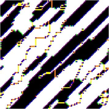
Motivations.                     Zero-point entropy on the pyrochlore lattice

    Geometrical frustration            �
                        Pyrochlore lattice = corner-sharing tetrahedra

     in spin ice        H     =
                                 J �
                                       �
                                          �
                                             σ
                                               �                            2

                                             pyro                       i
                                                      2   tet   i∈tet

 Pyroclhore lattice                    �   Pauling estimate of ground state
 + magnetic moments                        entropy S0 = ln Ngs :
                                                      �      �N/2
                                                          6            N 3
                                           Ngs = 2N              ⇒ S0 = ln
                                                          16           2 2

                                       �   microstates vs. constraints;
                                           N spins, N/2 tetrahedra
classical Ising spins pointing in the local direction = connect a site with the center of its tetrahedron

          FM nn and dipolar interactions       ⇒          GS: 2 in-2 out (ice-rules)

                                                                        Geometrically frustrated
                                                                            Ferromagnet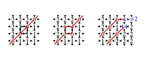
Motivations.

   Magnetic monopoles in spin-ice                                 (Castelnovo et al. , Nature 2008)

                             Projection

               ⇒     Ice configurations   ≡ { qα = 0 }

     - Thermal excitations violating the ice rules = magnetic monopoles

     - Finite energy to separate two monopoles to infinity = deconfined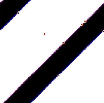
Motivations.

   Magnetic monopoles in spin-ice

                                                    Projection

 Experimental signatures:

   - Magnetic relaxation time give a dynamical signature of magnetic monopoles (Snyder et al., PRB 2004; Jaubert & Holdsworth, Nature
   Phys. 2009)

   - Current measurements    → extract magnetic charge in accordance with theory (Bramwell et al., Nature 2009)
   - Direct observation of magnetic monopoles? (induced current in a superconductor coil, Cabrera PRL 1982)

        →       Look for consequences rather than direct observations of Coulomb interaction between monopoles ...

                                                                                                                      1
Motivations.
2d spin ice model
At low T:
2 in - 2 out vertices only + bond distorsion (applied pressure)
Thermal excitations:
Vertices breaking the ice-rule are allowed but unfavoured = defects
16
�
square lattice
The model: +
binary variables on each edge
H= ni � i
i=1
Fix the Boltzmann weight of each of the i=1..16 local vertex configurations
• • • • • • • •
Integrability
(six- and eight-vertex models)
� �� � � �� � � �� � � �� �
a=ω1 =ω2 b=ω3 =ω4 c=ω5 =ω6 d=ω7 =ω8
• • • • • • • •
Non-Integrability
� �� �
Monte Carlo simulations
d=ω9 =ω10 =...=ω16
Spin ice behaviour: d � min(a, b, c)
Equilibrium phases of this general sixteen-vertex model?sed stepwise from above to below the coercive field. words, over 70% of all vertices had a spin-ice-like configuration. This
Motivations.
of the system after such field treatment revealed no excess percentage decreased monotonically with increasing lattice
esidual magnetic moment for the array, and a ten-fold spacing (decreasing interactions), approaching zero for our largest
2d spin ice model
the step dwell times did not significantly alter the
f vertex types described below.
lattice spacing, as would be expected for non-interacting (randomly
oriented) moments. In fact, the excess for all vertex types approached
zero as the lattice spacing increased, lending credence both to our
The model: understanding of the system and to the effectiveness of the rotating-
field method in enabling facile local re-orientation of the moments.
To further understand the nature of frustration in this system, we
also• studied• the pairwise correlations
16 between the Ising-like
• • • • • • �
moments of the islands. Defining a correlation function is somewhat
� �� � � �� � � �� � complicated
� H =naturenofi �our
�� by �the anisotropic i lattice and that of the
a=ω1 =ω2 b=ω3 =ω4 c=ω5 =ω6 d=ω7 =ω8
dipole interaction. We thus definei=1a set of correlation functions
between distinct types of neighbouring pairs. The closest pairing is
• • • • • • • •
� �� �
d=ω9 =ω10 =...=ω16
Experimental realizations:
- Experimentally realized by lithography: nanoarray of
ellongated ferromagnetic islands (Wang et al., Nature 2006).
ration -ofFerroelectricity (KDP,
frustration on the square water
lattice used inlayers
these in CFT...)
Each island in the lattice is a single-domain ferromagnet with
inting along the long axis, as indicated by the arrow. a, The
e lattice studied. The arrows indicate the directions of
sponding to the MFM image of Fig. 2b. b, Vertices of the Figure 2 | AFM and MFM images of a frustrated lattice. a, An AFM image
rs of moments indicated, illustrating energetically favourable of a typical permalloy array with lattice spacing of 400 nm. b, An MFM image
ble dipole interactions between the pairs. c, The 16 possible taken from the same array. Note the single-domain character of the islands,
urations on a vertex of four islands, separated into four as indicated by the division of each island into black and white halves. The
es. The percentages indicate the expected fraction of each moment configuration of the MFM image is illustrated in Fig. 1a. The
vidual moment orientations on an array were completely coloured outlines indicate examples of vertices of types I, II and III in pink,Equilibrium.
Equilibrium.

     Six-vertex model (exact results)
                                                                         b/c
     Ice-rules       ⇒d=0
      •          •            •           •           •          •
                                                                               FM
 �        ��         �    �        ��         �   �       ��         �
      a=ω1 =ω2                 b=ω3 =ω4               c=ω5 =ω6
                                                                                     PM
     Equilibrium phases:                                                  1         (critical)
        a 2 + b2 − c 2
     ∆=
             2ab                                                               AF                 FM
                                                                                                 (frozen)
     ∆>1                 freezed FM phase                                           1                       a/c
                 1rst order phase transition
     1 > ∆ > −1                   quasi long-range ordered PM phase
                              Kosterlitz-Thouless phase transition

     ∆ < −1               ordered AF phase with low energy excitations
Equilibrium.
Sixteen-vertex model (numerical results)
b/c
Allow defects ⇒ d �= 0
d�1
�
•
��
•
� �
•
��
•
� �
•
��
•
� �
•
��
•
�
FM
a=ω1 =ω2 b=ω3 =ω4 c=ω5 =ω6 d=ω7 =ω8
• • • • • • • •
� ��
d=ω9 =ω10 =...=ω16
�
1 PM 4d
Equilibrium phases: (disordered)
a2 + b2 − c2 − (4d)2 d�1 d�1
∆= FM
2(ab + c(4d)) AF (ordered)
∆ > 1 ordered FM phase 1 a/c
continuous phase transition
1 > ∆ > −1 disordered PM phase
continuous phase transition
∆ < −1 ordered
1 phase AF phase
→ agreement with exact results on the eight- and sixteen-vertex models for a
special choice of the parameters (Baxter PRL 1971, Wu PRL 1969)Out-of-equilibrium.
Out-of-equilibrium.                        200                                    200                                       200

hase-transition
                                                                    ’data’                                   ’data’                                   ’data’

   Phase ordering dynamics after a quench.  150                                    150                                       150

ated by symmetry, e.g. Ising magnets
      Evolution of the system across a phase transition.
                                            100                                    100                                       100

                                            50
                                                tendency to order in time BUT      50                                        50

                                            competition between two equivalent states                                       slow relaxation
                                             0
                                                  0   50
                                                           t=0
                                                            100   150        200
                                                                                    0
                                                                                         0   50
                                                                                                  t1 > 0
                                                                                                   100     150        200
                                                                                                                              0
                                                                                                                                   0
                                                                                                                                       t2 > t1
                                                                                                                                       50    100    150        200

                                            200                                    200                                       200

      !φ"
                                                                    ’data’                                   ’data’                                   ’data’

                                            150                                    150                                       150

                                            100                                    100                                       100

                                            50                                     50                                        50
                      T
rgy            Scalar order parameter        0
                                                  0   50    100   150        200
                                                                                    0
                                                                                         0   50    100     150        200
                                                                                                                              0
                                                                                                                                   0   50    100    150        200

       =⇒      The system   orders locally,
                        Question            giving rise
                                     : starting         to ordered
                                                     from          regions growing
                                                            equilibrium     at T0 in→
                                                                                    time.∞                                                  or     T0 = Tc
      - linear size of the domains     L(t)
                        equilibrium at Tf = Tc or Tf < Tc attained ?
      - the equilibration time diverges with the system size

            Dynamical scaling   ≡ only one lenght-scale in the system at large times (when domain growth)
                                   √
                          L(t) ∼        t
Out-of-equilibrium. 200 200 200
hase-transition
’data’ ’data’ ’data’
Phase ordering dynamics after a quench. 150 150 150
ated by symmetry, e.g. Ising magnets
Evolution of the system across a phase transition.
100 100 100
50
tendency to order in time BUT 50 50
competition between two equivalent states slow relaxation
0
0 50
t=0
100 150 200
0
0 50
t1 > 0
100 150 200
0
0
t2 > t1
50 100 150 200
!φ" ? 200
’data’
200
’data’
200
’data’
? 150 150 150
100 100 100
50 50 50
T
rgy Scalar order parameter 0
0 50 100 150 200
0
0 50 100 150 200
0
0 50 100 150 200
=⇒ The system orders locally,
Question giving rise
: starting to ordered
from regions growing
equilibrium at T0 in→
time.∞ or T0 = Tc
- linear size of the domains L(t)
equilibrium at Tf = Tc or Tf < Tc attained ?
- the equilibration time diverges with the system size
Dynamical scaling ≡ only one lenght-scale in the system at large times (when domain growth)
√
L(t) ∼ tOut-of-equilibrium.
Quench into the PM phase.
Same procedure in spin ice
• The presence of defects allows for single-spin flip dynamics, inplemented by a Continuous Time Monte Carlo algorithm.
• Prepare the system in a disordered equilibrium state and quench it into the ferromagnetic phase dominated by
type1 and 2 vertices (equivalent by symmetry)
b/c
initial configuration:
a = b = c = d = 1 (‘T=∞’) FM
at t=0 (instantaneously)
1 PM
a = b = c = 1, d � 1
AF FM
=⇒ • • • • • •
� �� � � �� � � �� �
a/c
a=ω1 =ω2 b=ω3 =ω4 c=ω5 =ω6
1
-
1
d/c
Magnetization = 0 BUT ‘close’ to a QLRO phase:Out-of-equilibrium.
Quench into the PM phase.
100
-1
The system gets trapped
10 in a metastable state with a
-2
eq d=10
-2
finite density of defects.
nd
10
10-3
Equilibration density
increases with d.
10-4 -2
10 102 106 1010 1014 10-2 102 106 1010 1014 It is equal to 2/N for
t (MCs) t (MCs) d < 10−4
L=50 L=100
The system lasts longer in the plateau for smaller d . ← Similar results in 3d dipolar spin-ice.
(Castelnovo et al., PRL 2010)
⇒ The presence of long-lived metastable states does not need long range dipolar interactions.Out-of-equilibrium.
Quench into the FM phase.
initial configuration: b/c
a = b = c = d = 1 (‘T=∞’)
at t=0 (instantaneously)
FM
−5 1 PM
a = 5, b = c = 1, d = 10 ( TOut-of-equilibrium.
Quench into the FM phase.
1 Rapid annihilation of defects
I II III IV
nd Growth of FM domains with walls
nc 120
0.75
nb L=300 || made of c-vertices and linked by
na
80
⊥
L=200 || strings.
L||,⊥(t)
⊥
Defects far from each other,
nκ(t)
L=100 ||
0.5 ⊥
40 t1/2 difficult to annihilate: slow dynamics.
0.25 0 Very stable domains
0 3 6
10 10 10
= Parallel bands
0
10-4 10-2 100 102 104 106 108 1010 1012
t (MCs)Out-of-equilibrium.
Quench into the FM phase.
Dynamic mechanisms
- anisotropy a≠b tends to create diagonal domain - once the bands are created we must create a pair of
walls made of AF vertices. defects and made them move along the walls to
- loop fluctuations are the elementary moves that do retore the equilibrium configuration. Extremely slow
not break the ice-rules. process.
- ‘corners’ of domains cannot have a neighbouring a-
vertex. Avoiding defects, this explains the presence of
strings.
- Strings connect two domains and mediate their
growth.Conclusion.
• Phase ordering kinetics of spin ice.
• → rich topological defects dynamics.
• Slow relaxation with long-lived density of
monopoles.
• Relaxation of a model «close» to
integrability.You can also read