Small Signal Interactions Involving a Synchronous Machine and a Grid Forming Converter
←
→
Page content transcription
If your browser does not render page correctly, please read the page content below
Small Signal Interactions Involving a Synchronous
Machine and a Grid Forming Converter
Luke Benedetti, Panagiotis N. Papadopoulos, Agustí Egea-Alvarez
Department of Electronic and Electrical Engineering
University of Strathclyde
Glasgow, UK
Luke.Benedetti@strath.ac.uk
Abstract—Interactions between synchronous machines (SMs) and implementations. However, there is limited research
and grid forming converters (GFMs) will become increasingly into the impact of these technologies on the stability of the
relevant as the power system transitions from a conventional power system as a whole.
fossil fueled synchronous based system to a renewable Small-signal analysis of GFMs in parallel connected to
generation rich and converter-based system. This paper
an infinite bus has been investigated in [8]. Additional small
investigates and confirms the possibility of electromechanical
signal analysis looking at robust stability margins using the
factor has been performed by the same authors in [9].
oscillatory modes between conventional SMs and converter
connected generation using a GFM control algorithm as well
as between two GFMs. The study employs small-signal models These papers look at synchronverters, a type of swing
and performs small-signal eigenvalue analysis. Moreover, equation based VSM, operating in parallel as well as
parametric sweeps are performed, to investigate the impact of synchronverters in parallel with GFLs.
network and GFM control parameters in controlling the A simplified frequency analysis for 100% CIG systems
electromechanical modes. has been outlined in [10]. The approach exploits similarities
between the SM and GFMs by allowing for the aggregation
Index Terms—Control, dynamics, electromechanical
oscillations, grid-forming converter, power electronics, power
of multiple machines. This is possible by considering the
systems, small signal stability, virtual synchronous machine. similarities between the swing equation and the GFM
control structure, which is different to the one used in this
I. INTRODUCTION study. However, they do not provide a small-signal analysis
of the electromechanical oscillations themselves.
The urgency associated with climate action is well
A detailed small-signal analysis has been performed in
understood, and the acceleration of the integration of
[11]. In this study the authors use eigenvalue analysis to
renewable energy sources (RESs) within the electricity grid
determine when a system comprised of two machines (all
is becoming a necessity if global temperature levels are to
combinations of SMs, GFLs and GFMs) become unstable
remain within acceptable levels [1]. Power converters are
with increasing penetrations of the CIG based machine (and
required to interface most RESs to the electricity system and
of the GFL specifically in the GFM-GFL case). It is seen
due to their very different characteristics, can potentially
from participation factor analysis that there are destabilising
introduce stability issues related to the reduction of inertia,
interactions between the fast voltage control of the
voltage and frequency regulation, and loss of synchronizing
converters and the relatively slow voltage control of the PSS
torque [2], amongst other challenges. GFMs are one of the
and AVR of the SM. It is also found that as GFL penetration
recommended approaches to facilitate the transition from
increases there reaches a point where there is not enough
conventional synchronous generation to converter
contribution from the SM (or GFM) to slow the frequency
interfaced generation (CIG).
variations and therefore the phase-locked loop (PLL) of the
GFM is a term incorporating a grid-tied converter
GFL loses synchronism. They also explore the impact of
controlled with the specific inclusion of voltage and
transmission line dynamics and the power system operating
frequency regulation [3]. This is different from the grid
point and expand their study to larger systems: first the
following converters (GFLs) which track the voltage signal
IEEE-9 bus and then a modified version of the South-East
and inject the specified power. There is a broad range of
Australian network. However, again, electromechanical
control philosophies under the GFM heading, each with
modes involving GFMs are not discussed in detail.
several different implementations and benefits. Some of the
From the literature, it can be determined that with the
most popular schemes currently within the literature include
inclusion of GFMs, further consideration to dynamic
droop control [4], virtual oscillator control (VoC) [5] and
interactions needs to be given, since new instability
the classification most similar to the generic GFM used in
mechanisms might appear in a complex power system.
this investigation, the VSM [6].
Therefore, considering power systems will most probably
There are several references in the literature,
involve SMs for years to come, the interactions between
investigating the impact of a high penetration of CIG on
power systems [7], but these are typically looking at grid- The work of Luke Benedetti was supported by an EPSRC Student
Excellence Award Studentship. The work of Panagiotis Papadopoulos was
following converters as opposed to GFMs. In addition, there supported by a UKRI Future Leaders Fellowship (grant number:
are several references describing different GFM approaches MR/S034420/1). All results can be fully reproduced using the methods and
data described in this paper and provided references.
978-1-6654-3597-0/21/$31.00 ©2021 IEEE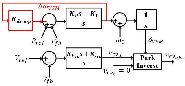
CIG and SMs should be well understood. Additionally, with highly nonlinear and complex. Therefore, it must first be
GFMs being recognised as a potential solution for linearised around the steady state operating point. First, the
maintaining stability, interactions specifically between SMs DAEs of the system are arranged in state-space form as,
and GFMs should be studied carefully. x =Ax+Bu=f(x,u) (1)
The fact that GFMs control active power through the
voltage angle, and have a resultant inherent frequency y=Cx+Du=g(x,u) (2)
synchronization, suggests the possibility of
electromechanical interactions between multiple machines where x is the vector of state variables and u and y the
[10]. Therefore, in this paper an initial investigation into vectors for the inputs and outputs, respectively. The dot
interactions between a GFM and an SM as well as between above the state vector in (1) suggests differentiation with
two GFMs is performed. To the extent of our knowledge, respect to time. A is the state matrix, B is the control matrix,
this particular interaction has not been investigated,
C is the output matrix and D is the feedforward matrix.
excluding qualitative recognition that this phenomenon is to
The linearisation is then achieved by introducing a small
be expected. Moreover, the impact of GFM control gains
and transmission line lengths on such oscillatory modes and disturbance, denoted by the prefix Δ, performing the Taylor
interactions between SMs and GFMs is also investigated in series expansion and then discarding all terms above first
this paper. It should be noted that the EMT implementation order, resulting in small deviation equations of the form,
Δx i =
of the models in this work allow for easier adaptation for ∂fi ∂fi ∂fi ∂fi (3)
Δx1 +…+ Δxn + Δu1 +…+ Δu
future investigations into more complicated or detailed ∂x1 ∂xn ∂u1 ∂ur r
systems and components, despite this level of detail not
being necessary to identify electromechanical modes of ∂gk ∂g ∂g ∂g (4).
oscillation. This future adaptability was considered because Δyk = Δx1 +…+ k Δxn + k Δu1 +…+ k Δur
∂x1 ∂xn ∂u1 ∂ur
high frequency phenomena have been proven to be
significant in the stability of systems with substantial levels It should be noted that intermediate steps for
of CIG [8], [11], [12]. This paper is mainly interested in understanding have been omitted but the full procedure can
investigating electromechanical modes, hence a relatively be found in [13].
simple (low order) SM model is used. However, a series of
high frequency oscillatory modes closely associated with B. Component Modelling
transmission line dynamics are also identified, one of which The component models included in this investigation are
is found to be of interest in terms of stability limits. This a SM, a GFM, RL branch transmission lines and a static
investigation, and the SM model used within, is considered constant impedance RL load.
a preliminary step applied on a smaller system to more
easily identify and investigate such interactions. A modular 1) Modelling Convention
modelling approach is adopted to allow for easy expansion The state-space equations are derived in the dq0 frame
to lager systems and higher order SM model as part of future with each machine operating in its own reference frame
work. dependent on its rotor angle, or virtual rotor angle for the
The remainder of this paper is structured as follows: GFM. The common reference frame can be chosen in one
section II describes the modelling of the network of two ways. The first is to determine the ‘centre of inertia’
components and details the layout of the system; section III and the second is to simply chose a machine to be the
discusses the results and analysis of the performed reference. The second approach was adopted for this
simulations and section IV provides the conclusions. investigation because it offers easier implementation with
no requirement to parameterise the inertia constant and
II. METHODOLOGY AND MODELLING
damping of the GFM. Additionally, the second approach
The small signal modelling in this work involves avoids the resultant redundant eigenvalue of the first
identifying the nonlinear state-space models of each approach [13].
component and considering how they connect together to Since the whole model is implemented in dq0 terms,
form a wider network. The differential algebraic equations whenever a Park transform would have been required to
(DAEs) associated with each component are then linearised transform signals in the abc-frame to the dq0-frame, there
and connected to form a single full network small signal is instead a simple vector rotation dependent on the angle
model (SSM). This section briefly describes the between the two dq0 frames. The same is true for any
linearisation process and then proceeds to detail the models instance of an inverse Park transform.
of each component used within this study. Several different modules within the network contain
A. Linearisation Process series RL or parallel capacitive components. In the balanced
A common approach to study electromechanical (and dq0 frame, these can be realised with equations:
idq = v1 dq − v2dq − +jω idq
1 R (5)
any other relevant) modes associated with a machine or
interactions between multiple machines is to perform a L L
small-signal analysis. To achieve this, the system being
analysed must be linear, but power systems are known to be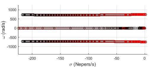
vdq = idq − i2dq − jωvdq
1 (6) of pulse width modulation (PWM). An inverse Park
C transform is used to translate the converter voltage and
angle from the control scheme directly into the voltage at
where the currents, voltages, resistance, and inductance are the output of the converter. There is also a harmonic filter
displayed in figure 1. Note, the subscript ‘dq’ denotes the containing a series RL impedance followed by a parallel
phasor represented by d and q components as = − capacitance at the GFM output terminal. This is of the
. The equations for the RL and the C segments can be configuration seen in figure 1. and modelled in accordance
extracted and used separately depending on the with (5) and (6).
configuration. For example, the transmission lines are The control structure of the GFM contains two main
implemented as simple RL impedances modelled in loops. The first is the power loop which manipulates the
accordance with (5) but neglecting the capacitive dynamics virtual rotor speed, and hence angle, with a PI controller
described by (6). acting on the difference between the reference power Pref
and the measured (or feedback) power Pfb . This is the same
principle as the SM swing equation and the two systems can
be directly compared in their second order dynamic
responses by looking at the characteristic equation of their
transfer functions. This allows for the equivalent inertia and
damping values to be described in terms of the PI controller
gains, and . From this it is found that impacts inertia
Figure 1. RLC circuit diagram. while both and impact damping. However, it can be
2) Synchronous Machine noted that there are differences in the steady state response
The SM model comprises the swing equation along with since the PI controller acts to bring the output power exactly
an RL impedance but neglects rotor dynamics as in this to its reference, that is there is no damping feedback term
paper we are focusing on identifying oscillatory modes in acting on the change of rotor speed as there is in the swing
the electromechanical range. The swing equation captures equation (although the red droop branch in fig. 2 essentially
the relationship between the SM rotor speed (and hence solves this). The second loop is the voltage loop, acting as
angle) and the difference between the input mechanical and an AVR by maintaining the voltage magnitude at the
output electrical power. This relationship can be written as, filtering capacitor, Vfb , to the reference value, Vref .
1
ω = P − P − K Δω − K Δω
(7) In the test case with only GFMs, described later, one of
2H the machines is also equipped with frequency droop control
δr =ωr
to balance the active power in the system. The block
(8), diagram for the GFM control structure is displayed in fig. 2.
Note, the frequency droop branch (displayed in red) is only
where ωr and δr are the rotor speed and angle, respectively. present for one of the machines in the only-GFM test case,
The damping coefficient is termed KD and the inertia for better equivalence to the SM-GFM test case.
constant, H. Finally, the mechanical and electrical powers
are denoted by Pm and Pe , respectively. A speed governor
has been included which has been simplified to a
proportional gain, Kgov , acting on a change of rotor speed to
augment the mechanical input power.
The electrical part of the SM model consists of the
resistance and inductance resulting from the armature coils
in addition to the inductance attributed to the armature
reaction. The combined impedance is termed the
synchronous impedance, Zs =Rs +jXs , with Rs being the
armature resistance and Xs combining the effects of the
armature leakage inductance and armature reaction. The Figure 2. GFM control scheme block diagram.
transformation from the SM dq0-frame to the common dq0-
frame is performed behind the synchronous impedance. 4) Static Load
However, there is a possible alternative whereby the The load is modelled as a constant RL impedance. The
transformation is performed at the SM terminals (after the values of the resistance and inductance are calculated with
Rload = nP
synchronous impedance). This synchronous impedance is V2 (9)
modelled dynamically, in accordance with (5). load
3) Grid Forming Converter
(ω ×Q )
The power converter section of the GFM is represented V2n (10),
Lload =
with an averaged model which neglects switching effects 0 load
and the time delay usually associated with the employment
where Vn is the base voltage and ω0 is the base electrical ψij × ϕij
n
∑i=1 | ψij |× ϕij
frequency. The desired load active and reactive powers are pij = (11)
denoted by Pload and Qload , respectively.
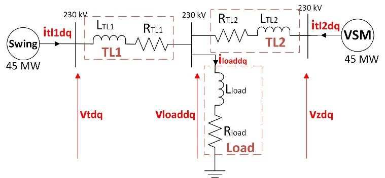
C. Systems Under Study
where ψ and ϕ are the left and right eigenvectors,
Two networks with the layout in fig. 3 are analysed in respectively.
this work. The ‘swing’ machine being the SM in one test Finally, parametric sweeps are performed to determine
case and the droop-augmented GFM in the other. Further the impact on the small-signal stability of different network
signals within the machines include icvdq which is the elements such as transmission line lengths or GFM controls.
current through the RL section of the GFM output filter and The parameters associated with each test case are displayed
ismdq which is simply equivalent to itl1dq in this case. in table i. The GFM parameters are common to both
machines in the only-GFM network with the swing machine
also having a droop parameter of Kdroop =0.5100 ×10⁶ .
Additionally, vcvdq is the voltage behind the filter impedance
in the GFM and Edq is the internal generated voltage of the
SM. In the GFM-GFM network, all GFM specific TABLE I. NETWORK PARAMETERS.
parameters or signals are given a subscript of ‘1’ if related GFM
SM Parameter Value Value
to the left machine or ‘2’ if related to the right. The Parameter
modularity of the networks is achieved through H 4 KP 9×10⁻⁹
development of state space models for each component KD +Kgov ≅10 KI 4×10⁻⁸
separately (including individual transmission line RS 10.58 Ω KPVC 0.1
branches). Following this, the interconnection of signals is
LS 0.5052 H KIVC 50
achieved with an additional module pertaining to voltage
Pm 50 MW Rf 5.29 Ω
specification and Kirchhoff’s current law for each bus.
Finally, the initial states required for the SSMs were Vref 230 kV Lf 0.1347 H
obtained using a power flow analysis with the aid of Network
Value Cf 1 μF
MATPOWER to solve the steady-state equations. Parameter
RTL1=RTL2 35.688 Ω Pref 50 MW
LTL1=LTL2 0.1272 H Vref 230 kV
III. RESULTS AND ANALYSIS
A. SM-GFM Network Eigenvalue Analysis
The procedure explained above is performed for the
network containing the SM and GFM combination. The
eigenvalues are presented in table ii. This table also
includes the frequency of the mode and the corresponding
Figure 3. Final network layout single line diagram. damping ratio. Using this information, the
The SSMs have been validated by comparing step electromechanical mode is identified as λ9 & λ10 . Following
responses with corresponding Simulink models. this, the participation factors representing the contribution
of each state to each oscillatory mode were calculated and
D. Small Signal Analysis
those with significant contribution (>10%) were added to
For both network configurations being tested, small-signal the table.
analysis utilising eigenvalues is performed. The use of
TABLE II. SM-GFM-LOAD SYSTEM EIGENVALUES.
eigenvalue analysis [13] offers insight into the oscillatory
modes that might be excited after a disturbance such as a Damping Contributing
Eigenvalues Value Frequency States
Ratio
load increase. With this, potential electromechanical modes
-9.56 ·103 ismdq , itl2 dq
can be identified by calculating the frequency of the modes λ1 & λ2 13.396 kHz 11.28 %
±j8.42·104
and extracting those in the proximity of up to 3 Hz.
λ3 & λ4 -77.07±j3843 612 Hz 2.01 % vzdq , icvdq
Typically, with SMs, local modes are in the range of 1 to 3
Hz and interarea modes are less than 1 Hz [14]. The λ5 & λ6 -52.38±j3043 484 Hz 1.72 % vzdq , icvdq
eigenvalues and associated frequency and damping ratio are
obtained as in [13]. The next step is to calculate the −216.15 icvdq , ismdq ,
λ7 & λ8 115 Hz 28.65 %
±j722.71 itl2 dq
participation factor of each state for each mode. This gives
-1.5661
an idea of which states are the most involved in specific λ9 & λ10 1.68 Hz 14.65 % ωr , δGFM
±j10.57
oscillatory modes and is especially useful in identifying
interactions between two machines. The calculation, from The most significant states in contributing to the
[14], is electromechanical mode are ωr and δGFM . This clearly
suggests an interaction between the SM and GFM,
confirming the expected behaviour. This information is                                 TABLE III.       GFM-GFM-LOAD SYSTEM EIGENVALUES.
useful in considering future control of power systems.                                                                         Damping     Contributing
Techniques previously used to address interactions between                       Eigenvalues         Value       Frequency                   States
                                                                                                                                Ratio
SMs will likely need to be considered as GFM-coupled                                              -9.51·103        13.303                  itl1dq , itl2 dq
                                                                                    λ1 & λ2                                    11.31 %
RESs are integrated.                                                                              ±j8.36·104        kHz
     High frequency oscillatory modes are also present, the                         λ3 & λ4       -73.7±j4271     680 Hz        1.73 %      vz1dq ,vz2dq
most interesting being λ3 to λ6 which are seen to have very                         λ5 & λ6       -75±j3636       579 Hz        2.06 %      vz1dq ,vz2dq
low damping. Despite the low damping ratio associated
                                                                                                                                            vz1d , icv1d
with some of these modes, they are damped very quickly in                           λ7 & λ8      -12.46±j3065     488 Hz        0.41 %
                                                                                                                                            vz2d , icv2d
time. The damping ratio represents attenuation of the mode                                                                                  vz1q , icv1q
per cycle and with high frequency, the oscillation does not                         λ9 & λ10     -14.52±j2514     400 Hz        0.58 %
                                                                                                                                            vz2q , icv2q
last long in time. Through parametric sweeps (excess to
                                                                                   λ11 & λ12     -155.1±j316.5    50.4 Hz       44 %       itl1dq , itl2 dq
those in the scope of this paper), the eigenvalues of λ3 to λ6
were affected by the GFM voltage loop controls as well as                                                                                     Pint1 ,
                                                                                   λ13 & λ14        -2.8±j3.7     0.589 Hz      60.4 %
the transmission line lengths, as expected from the                                                                                        Pint2 ,δVSM2
contributing states which includes a small participation
from the voltage loop integrator state, Vint , of 0.19 % for λ3                 equivalent to those in the SM-GFM network but with the
& λ4 and 0.27 % for λ5 & λ6 .                                                   addition of two oscillatory modes denoted in this network
     The very fast oscillatory mode of 13.396 kHz was only                      by λ7 to λ10 . These are found to have similar characteristics
found to be affected by the transmission line length and not                    to λ3 to λ6 for both networks.
by any of the GFM control gains. Also, the remaining mode                       C. Parametric Sweeps
of 115 Hz is discussed later with the KP parametric sweep.                      To further the contribution of this work, parametric sweeps
B. GFM-GFM Network Eigenvalue Analysis                                          were performed for several different network and control
     In a similar manner, the eigenvalues and corresponding                     parameters to determine their impact on the oscillatory
attributes for the GFM-GFM network are presented in table                       modes.
III. The electromechanical mode is this time identified to be                   The eigenvalues of interest are displayed with non-essential
λ13 & λ14 . Again, the participation factors are calculated and                 modes being omitted. The first investigation increased the
contributing states of each mode are shown in table iii. The                    lengths of the transmission lines. The resistance and
states with the highest contribution to the electromechanical                   reactance per kilometer of both lines are chosen by
modes are found to be Pint1 , Pint2 , and δVSM2 . These states                  calculating the required rated current and selecting from the
are associated with the active power loops of the GFMs and                      relevant table of cable sizes [15]. Fig. 4a displays the result
suggest an electromechanical interaction. High frequency                        of varying the TL1 and TL2 lengths from 40 to 120 km
modes are also present in this network with analysis being                      simultaneously. The next two investigations are performed

                                (a)                                                     (b)                                    (c)

                                             (d)                                                         (e)

                                             (f)                                                      (g)
    Figure 4. Eigenvalues of interest for parametric sweep of the SM-GFM-load network for (a) TL1 & TL2, (b) KP, (c) zoomed KP, (d) KI and of the
                                               GFM-GFM-load network for (e) KP1 , (f) KI1 and (g) Kdroop.
for the GFM power loop PI controller gains. The plots for GFM network, it was found that the PI control gains of the
the proportional gain, KP , and integral gain, KI , are droop-augmented GFM provided the potential to fully
displayed in fig. 4b to 4c and fig. 4d, respectively. KP was damp the electromechanical interaction with no significant
swept from 0 to 1 ×10⁻⁶ and KI was swept from 1 ×10-12 to effect on any higher frequency oscillations. However,
1 ×10⁻⁵ . The same sweeps are performed in the GFM-GFM increasing the frequency droop gain brought the
case and similar trends are observed; therefore, these have electromechanical mode closer to the unstable region,
not been presented here. Additionally, the PI gains of the similar to increasing the transmission line lengths.
power loop for the droop-augmented-GFM were swept with REFERENCES
the same range as in the other GFM. These sweeps are
displayed in fig. 4e and fig. 4f. Finally, the impact of the [1] International Panel on Climate Change (IPCC), "Special Report:
frequency droop gain, Kdroop , is investigated. This Global Warming of 1.5 Degrees Celcius Summary for Policy
Makers," IPCC, Geneva, 2018.
parametric sweep is displayed in fig. 4g and ranges from 0
[2] F. Milano, F. Dörfler, G. Hug, D. J. Hill and G. Verbič,
to 10(100 ×106 ). "Foundations and challenges of low-inertia systems (invited
1) SM-GFM Network Parametric Sweep Results paper)," in 2018 Power Systems Computation Conference (PSCC),
When analysing fig. 4a, it is seen that with an increasing Dublin, 2018.
length, the damping ratio of the electromechanical mode [3] M. Paolone, T. Gaunt, X. Guillaud, M. Liserre, S. Meliopoulos, A.
Monti, T. Van Cutsem, V. Vijay and C. Vournas, "Fundamentals of
decreases from 16.84 % to 12.88 %. In this test case the
power systems modelling in the presence of converter-interfaced
mode remains stable but in a different system, the impact of generation," Electric Power Systems Research, vol. 189, p. 106811,
transmission line length might be more critical. 2020.
Altering the controller gains shows significant impact on [4] X. Meng, K. Liu and Z. Liu, "A generalized droop control for grid-
the electromechanical mode in fig. 4c and fig. 4d. The gain supporting inverter based on comparison between traditional droop
KI is seen to cause small-signal instability of the control and virtual synchronous generator control," IEEE
Transactions on Power Electronics, vol. 34, no. 6, pp. 5416-5438,
electromechanical mode as it is increased whereas KP can 2019.
fully damp the interaction, however the oscillation at [5] M. Liu, S. Dutta, V. Purba, S. Dhople and B. Johnson, "A grid-
115 Hz, seemingly related to network current dynamics, is compatible virtual oscillator controller: analysis and design," in
brought towards the unstable region, as seen in fig. 4b. 2019 IEEE Energy Conversion Congress and Exposition (ECCE),
2) GFM-GFM Network Parametric Sweep Results Baltimore, MD, 2019.
The increase of the proportional and integral gains, KP1 [6] H. P. Beck and R. Hesse, "Virtual synchronous machine," in 2007
9th International Conference on Electrical Power Quality and
and KI1 , are seen to fully damp the electromechanical Utilisation, Barcelona, 2007.
interaction and this time no adverse effect is found on any [7] C. Collados-Rodriguez, M. Cheah-Mane, E. Prieto-Araujo and O.
higher frequency modes. The droop gain sweep in fig. 4g Gomis-Bellmunt, "Stability analysis of systems with high VSC
provides evidence of another highly impactful control penetration: where is the limit?," IEEE Transactions on Power
Delivery, vol. 35, no. 4, pp. 2021-2031, 2019.
parameter associated with the GFM, allowing for higher
[8] R. Rosso, S. Engelken and M. Liserre, "Analysis of the behavior of
controllability of the electromechanical mode dynamics. synchronverters operating in parallel by means of component
Like the transmission line length sweep, it is seen that the connection method (CCM)," in 2018 IEEE Energy Conversion
electromechanical mode is brought towards the unstable Congress and Exposition (ECCE), Portland, OR., 2018.
region, potentially causing instability if this mode was [9] R. Rosso, S. Engelken and M. Liserre, "Robust stability analysis of
initially closer to the y-axis. synchronverters operating in parallel," IEEE Transactions on Power
Electronics, vol. 34, no. 11, pp. 11309-11319, 2019.
IV. CONCLUSIONS [10] G. S. Pereira, V. Costan, A. Bruyére and X. Guillaud, "Simplified
This paper presents a preliminary investigation into approach for frequency dynamics assessment of 100% power
electronics-based systems," Electric Power Systems Research, vol.
interactions between SMs and GFMs with a focus on 188, p. 106551, 2020.
electromechanical modes. This is achieved with modular
[11] U. Markovic, O. Stanojev, P. Aristidou, E. Vrettos, D. S. Callaway
small-signal modelling, followed by eigenvalue analysis. and G. Hug, "Understanding Small-Signal Stability of Low-Inertia
The states corresponding to the electromechanical mode in Systems," IEEE Transactions on Power Systems.
the SM-GFM system were found to be those associated with [12] J.-S. Brouillon, M. Colombino, D. Gross and F. Dörfler, "The effect
the power loop of the GFM and the swing equation of the of transmission-line dynamics on globally synchronizing controller
SM, thereby confirming the presence of electromechanical for power inverters," in 2018 7th European Control Conference
(ECC), Limassol, 2018.
interactions, similarly between two GFMs. Finally, a series
[13] P. Kundur, Power System Stability and Control, New York:
of parametric sweeps are performed, offering an insight into McGraw-Hill, 1994.
the impact and flexibility that the GFM control provides for
[14] P. W. Sauer and M. A. Pai, Power System Dynamics and Stability,
manipulating the electromechanical mode. Urbana: Upper Saddle River, NJ, 1997.
Small-signal instability is found to occur from high
values of as the electromechanical mode traverses into
[15] M. Reta-Hernandez, "Chapter 13 - Transmission Line Parameters,"
the unstable region. In the case of , this mode can be fully
in Electric Power Generation, Transmission, and Distribution, Boca
Raton, FL, CRC Press, 2012.
damped but doing so will bring a higher frequency
oscillation towards instability. Additionally, for the GFM-You can also read