State of the Global Climate 2020 - WMO-No. 1264 - WMO Library
←
→
Page content transcription
If your browser does not render page correctly, please read the page content below
State of the
                        Global Climate
                        2020
WEATHER CLIMATE WATER

                                         WMO-No. 1264
WMO-No. 1264
© World Meteorological Organization, 2021

The right of publication in print, electronic and any other form and in any language is reserved by WMO.
Short extracts from WMO publications may be reproduced without authorization, provided that the complete source
is clearly indicated. Editorial correspondence and requests to publish, reproduce or translate this publication in
part or in whole should be addressed to:

Chair, Publications Board
World Meteorological Organization (WMO)
7 bis, avenue de la Paix                                              Tel.: +41 (0) 22 730 84 03
P.O. Box 2300                                                         Fax: +41 (0) 22 730 81 17
CH-1211 Geneva 2, Switzerland                                         Email: publications@wmo.int

ISBN 978-92-63-11264-4

Cover illustration: Central photo: Dry grass wildfire caused by arson started a larch forest fire near Srednekolymsk, Sakha Republic, Russia, 24 June
2020. Contains modified Copernicus Sentinel data 2020. Photo credits: Pierre Markuse

NOTE

The designations employed in WMO publications and the presentation of material in this publication do not imply the expression of any opinion
whatsoever on the part of WMO concerning the legal status of any country, territory, city or area, or of its authorities, or concerning the delimitation
of its frontiers or boundaries.

The mention of specific companies or products does not imply that they are endorsed or recommended by WMO in preference to others of a similar
nature which are not mentioned or advertised.

The findings, interpretations and conclusions expressed in WMO publications with named authors are those of the authors alone and do not necessarily
reflect those of WMO or its Members.

 B
Contents
Foreword .  .  .  .  .  .  .  .  .  .  .  .  .  .  .  .  .  .  .  .  .  .  .  .  .  .  .  .  .  .  .  .  .  .  .  .  .  .  .  .  .  .  .  .  .  .3

Foreword by the United Nations Secretary-General .  .  .  .  .  .  .  .  .  .  .  .  .  .  .  .  .  .  .  .  .  .4

Highlights .  .  .  .  .  .  .  .  .  .  .  .  .  .  .  .  .  .  .  .  .  .  .  .  .  .  .  .  .  .  .  .  .  .  .  .  .  .  .  .  .  .  .  .  .  .5

Global climate indicators .  .  .  .  .  .  .  .  .  .  .  .  .  .  .  .  .  .  .  .  .  .  .  .  .  .  .  .  .  .  .  .  .  .  .  .  .6

    Temperature  .  .  .  .  .  .  .  .  .  .  .  .  .  .  .  .  .  .  .  .  .  .  .  .  .  .  .  .  .  .  .  .  .  .  .  .  .  .  .  .  .  . 6

    Greenhouse gases and stratospheric ozone  .  .  .  .  .  .  .  .  .  .  .  .  .  .  .  .  .  .  .  .  .  .  .  .  .8

    Ocean  .  .  .  .  .  .  .  .  .  .  .  .  .  .  .  .  .  .  .  .  .  .  .  .  .  .  .  .  .  .  .  .  .  .  .  .  .  .  .  .  .  .  .  .  . 10

    Cryosphere  .  .  .  .  .  .  .  .  .  .  .  .  .  .  .  .  .  .  .  .  .  .  .  .  .  .  .  .  .  .  .  .  .  .  .  .  .  .  .  .  .  . 15

         The Arctic in 2020 .
                       2020  .  .  .  .  .  .  .  .  .  .  .  .  .  .  .  .  .  .  .  .  .  .  .  .  .  .  .  .  .  .  .  .  .  .  .  .  . 18

    Precipitation .  .  .  .  .  .  .  .  .  .  .  .  .  .  .  .  .  .  .  .  .  .  .  .  .  .  .  .  .  .  .  .  .  .  .  .  .  .  .  .  .  . 21

    Drivers of short-term climate variability .  .  .  .  .  .  .  .  .  .  .  .  .  .  .  .  .  .  .  .  .  .  .  .  .  . 22

    A year of widespread flooding, especially in Africa and Asia .  .  .  .  .  .  .  .  .  .  .  .  .  .  . 23

High-impact events in 2020 .  .  .  .  .  .  .  .  .  .  .  .  .  .  .  .  .  .  .  .  .  .  .  .  .  .  .  .  .  .  .  .  .  .  . 23

    Heatwaves, drought and wildfire  .  .  .  .  .  .  .  .  .  .  .  .  .  .  .  .  .  .  .  .  .  .  .  .  .  .  .  .  .  . 24

    Extreme cold and snow  .  .  .  .  .  .  .  .  .  .  .  .  .  .  .  .  .  .  .  .  .  .  .  .  .  .  .  .  .  .  .  .  .  .  . 26

    Tropical cyclones .  .  .  .  .  .  .  .  .  .  .  .  .  .  .  .  .  .  .  .  .  .  .  .  .  .  .  .  .  .  .  .  .  .  .  .  .  .  . 27

    Extratropical storms  .  .  .  .  .  .  .  .  .  .  .  .  .  .  .  .  .  .  .  .  .  .  .  .  .  .  .  .  .  .  .  .  .  .  .  .  . 29

         Climate indicators and sustainable development goals  .  .  .  .  .  .  .  .  .  .  .  .  .  .  .  . 31

         Observational basis for climate monitoring .
                                         monitoring .  .  .  .  .  .  .  .  .  .  .  .  .  .  .  .  .  .  .  .  .  .  . 32

Risks and impacts  .  .  .  .  .  .  .  .  .  .  .  .  .  .  .  .  .  .  .  .  .  .  .  .  .  .  .  .  .  .  .  .  .  .  .  .  .  .  .  . 34

    Human mobility and displacement  .  .  .  .  .  .  .  .  .  .  .  .  .  .  .  .  .  .  .  .  .  .  .  .  .  .  .  .  . 34

    Compounded crisis impacts on food security, displacement, and humanitarian action 38

         Clean energy, disaster-proof infrastructure and early warning systems  .  .  .  .  .  .  . 42

         Case study 1: Protecting farmers in Pakistan from the compounded
         impacts of severe weather, locusts and COVID-19  .  .  .  .  .  .  .  .  .  .  .  .  .  .  .  .  .  .  . 45

         Case study 2: Forecast-based financing and anticipatory action in Bangladesh .
                                                                           Bangladesh .  .  . 45

Data set details  .  .  .  .  .  .  .  .  .  .  .  .  .  .  .  .  .  .  .  .  .  .  .  .  .  .  .  .  .  .  .  .  .  .  .  .  .  .  .  .  . 46

List of contributors  .  .  .  .  .  .  .  .  .  .  .  .  .  .  .  .  .  .  .  .  .  .  .  .  .  .  .  .  .  .  .  .  .  .  .  .  .  .  . 51

                                                                                                                                                       1
Since 2016, the following United Nations agencies have significantly
    contributed to the WMO State of the Global Climate publication
    in support of climate policy and action:

        Food and Agriculture Organization of the United Nations (FAO),

        Intergovernmental Oceanographic Commission
        of the United Nations Educational, Scientific and Cultural
        Organization (IOC-UNESCO),

        International Monetary Fund (IMF),

        International Organization for Migration (IOM),

        Office of the United Nations High Commissioner
        for Refugees (UNHCR),

        United Nations Environment Programme (UNEP),

        World Food Programme (WFP),

        World Health Organization (WHO).

    WMO also recognizes the substantial contributions that many
    non-United Nations organizations have made to this report.
    For a list of all the contributors to this report, see List of contributors.

2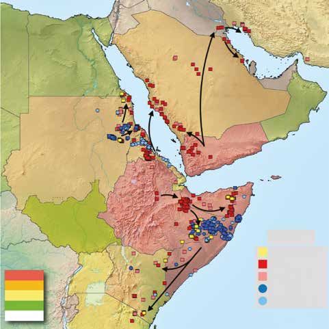
Foreword
                                                  Concentrations of the major greenhouse
                                                  gases continued to increase in 2019 and
                                                  2020. Globally averaged mole fractions of
                                                  carbon dioxide (CO2) have already exceeded
                                                  410 parts per million (ppm), and if the CO2
                                                  concentration follows the same pattern as
                                                  in previous years, it could reach or exceed
                                                  414 ppm in 2021.

                                                  Stabilizing global mean temperature at 1.5 °C
                                                  to 2 °C above pre-industrial levels by the
                                                  end of this century will require an ambitious
                                                  reduction of greenhouse gas emissions, which
                                                  must begin to occur during this decade.

                                                  I take this opportunity to congratulate the
                                                  experts and the lead author, who compiled
                                                  this report using physical data analyses and
It has been 28 years since the World Mete-        impact assessments. I thank all the contrib-
orological Organization issued the first state    utors, particularly WMO Member National
of the climate report in 1993. The report was     Meteorological and Hydrological Services
initiated due to the concerns raised at that      and Regional Climate Centres and our sister
time about projected climate change. While        United Nations Agencies for their collabora-
understanding of the climate system and           tion and input on this report. The report is
computing power have increased since then,        intended to help our organizations to update
the basic message remains the same, and we        world leaders and citizens on the latest infor-
now have 28 more years of data that show          mation about our Earth system’s behaviour
significant temperature increases over land       and climate change impacts. WMO remains
and sea, as well as other changes, such as        committed to supporting this publication and
sea-level rise, melting of sea ice and glaciers   communicating it widely for this purpose.
and changes in precipitation patterns.

This underscores the robustness of climate
science based on the physical laws governing
the behaviour of the climate system. All key
climate indicators and impact information
provided in this report show relentless,
continuing climate change, an increasing
occurrence and intensification of high-im-
pact events and severe losses and damages                          (P. Taalas)
affecting people, societies and economies.                     Secretary-General

                                                                                                    3
Foreword by the United Nations
    Secretary-General
                                                     We know that to avert the worst impacts of
                                                     climate change, we must keep global temper-
                                                     atures to within 1.5 °C of the pre-industrial
                                                     baseline. That means reducing global green-
                                                     house gas emissions by 45 per cent from
                                                     2010 levels by 2030 and reaching net zero
                                                     emissions by 2050. The data in this report
                                                     show that the global mean temperature
                                                     for 2020 was around 1.2 °C warmer than
                                                     pre-industrial times, meaning that time is
                                                     fast running out to meet the goals of the
                                                     Paris Agreement. We need to do more, and
                                                     faster, now.

                                                     This year is pivotal. At the United Nations
                                                     climate conference, COP26, in November,
                                                     we need to demonstrate that we are taking
                                                     and planning bold action on mitigation and
    2020 was an unprecedented year for people        adaptation. This entails scaled-up financial
    and planet: a global pandemic on a scale         flows from developed to developing coun-
    not seen for more than a century; global         tries. And it means radical changes in all
    temperatures higher than in a millennium; and    financial institutions, public and private, to
    the highest concentration of carbon dioxide      ensure that they fund sustainable and resilient
    in our atmosphere for over 3 million years.      development for all and move away from a
                                                     grey and inequitable economy.
    While many will remember 2020 most poign-
    antly for how the COVID-19 pandemic affected     As the world focuses on COVID-19 recovery,
    the world, this report explains that, for many   let us use the opportunity to get back on track
    across the planet, especially in developing      to achieve the Sustainable Development Goals
    countries, 2020 was also a year of extreme       and reduce the threat from climate change.
    weather and climate disruption, fuelled by       I call on everyone – from governments, civil
    anthropogenic climate change, affecting lives,   society and business to individual citizens –
    destroying livelihoods and forcing many          to work to make 2021 count.
    millions from their homes.

    This report also demonstrates the impact of
    this warming, both on the planet’s ecosystems
    and on individuals and communities, through
    superstorms, flooding, heatwaves, droughts
    and wildfires. We know what needs to be
    done to cut emissions and adapt to climate
    impacts now and in the future. We have the
    technology to succeed. But current levels of
    climate ambition and action are significantly                   (A. Guterres)
    short of what is needed.                              United Nations Secretary-General

4
Highlights
    Concentrations of the major greenhouse gases, CO2, CH4, and N2O, continued
    to increase despite the temporary reduction in emissions in 2020 related
    to measures taken in response to COVID-19.

                        2020 was one of the three warmest years on record. The past
                        six years, including 2020, have been the six warmest years on
                        record. Temperatures reached 38.0 °C at Verkhoyansk, Russian
                        Federation on 20 June, the highest recorded temperature
                        anywhere north of the Arctic Circle.

                                     The trend in sea-level rise is accelerating.
                                     In addition, ocean heat storage and acidification
                                     are increasing, diminishing the ocean’s capacity
                                     to moderate climate change.

                                            The Arctic minimum sea-ice extent in
                                            September 2020 was the second lowest
                                            on record. The sea-ice retreat in the
                                            Laptev Sea was the earliest observed in
                                            the satellite era.

                                            The Antarctic mass loss trend accelerated
                                            around 2005, and currently, Antarctica loses
                                            approximately 175 to 225 Gt of ice per year.

                                     The 2020 North Atlantic hurricane season
                                     was exceptionally active. Hurricanes, extreme
                                     heatwaves, severe droughts and wildfires led
                                     to tens of billions of US dollars in economic
                                     losses and many deaths.

                        Some 9.8 million displacements, largely due to
                        hydrometeorological hazards and disasters, were
                        recorded during the first half of 2020.

    Disruptions to the agriculture sector by COVID-19 exacerbated weather
    impacts along the entire food supply chain, elevating levels of food insecurity.

                                                                                       5
Global climate indicators
                             Global climate indicators1 reveal the ways in              1981–2010 is used, where possible, as a base
                             which the climate is changing and provide a                period for consistent reporting of surface
                             broad view of the climate at the global scale.             measurements, satellite data and reanalyses.
                             They are used to monitor the key components                For some indicators, it is not possible to use
                             of the climate system and describe the most                this base period, either because there are
                             relevant changes in the composition of the                 no measurements in the early part of the
                             atmosphere, the heat that arises from the                  period, or because a longer base period is
                             accumulation of greenhouse gases (and                      needed to calculate a representative average.
                             other factors), and the responses of the                   Where the base period used is different from
                             land, ocean and ice to the changing climate.               1981–2010, this is noted in the text or figure
                             These indicators include global mean surface               captions, and more details are given in the
                             temperature, global ocean heat content, state              Data set details section.
                             of ocean acidification, glacier mass balance,
                             Arctic and Antarctic sea-ice extent, global
                             CO2 mole fraction and global mean sea level
                             and are discussed in detail in the sections                TEMPERATURE
                             below. Further information on the data sets
                             used for each indicator can be found at the                The global mean temperature for 2020 was
                             end of this report.                                        1.2 ± 0.1 °C above the 1850–1900 baseline
                                                                                        (Figure 1), which places 2020 as one of the
                             A variet y of baselines are used in this                   three warmest years on record globally. The
                             report. For global mean temperature, the                   WMO assessment is based on five global
                             baseline is 1850–1900, which is the baseline               temperature data sets (Figure 1). All five
                             used in the IPCC Special Report on Global                  of these data sets currently place 2020 as
                             Warming of 1.5 °C as an approximation of                   one of the three warmest years on record.
                             pre-industrial temperatures.2 For greenhouse               The spread of the five estimates of the an-
                             gases, pre-industrial concentrations estimated             nual global mean ranges between 1.15 °C
                             from ice cores for the year 1750 are used                  and 1.28 °C above pre-industrial levels (see
                             as baselines.                                              the baseline definition in the Global climate
                                                                                        indicators section). It is worth noting that
                             For other variables and for temperature maps,              the Paris Agreement aims to hold the global
                             the WMO climatological standard normal                     average temperature to well below 2 °C above

Figure 1. Global annual
mean temperature
difference from                                   HadCRUT analysis
pre-industrial conditions                1.2      NOAAGlobalTemp
(1850–1900) for five                              GISTEMP
                                         1.0
global temperature data
                                                  ERA5
sets. For details of the                 0.8      JRA-55
data sets and plotting,
see Temperature data                     0.6
                                   °C

in the Data set details
section at the end of this               0.4
report.
                                         0.2

                                         0.0

                                        –0.2

                                               1850         1875     1900        1925          1950       1975               2000               2025
                                                                                        Year                       © Crown Copyright. Source: Met Office

                             1
                                 https://journals.ametsoc.org/view/journals/bams/aop/bamsD190196/bamsD190196.xml
                             2
                                 http://www.ipcc.ch/sr15/

        6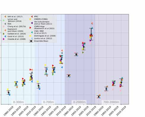
Figure 2. Temperature
                                                                                                               anomalies relative to
                                                                                                               the 1981–2010 long-term
                                                                                                               average from the ERA5
                                                                                                               reanalysis for 2020.
                                                                                                               Source: Copernicus
                                                                                                               Climate Change Service,
                                                                                                               European Centre for
                                                                                                               Medium-Range Weather
                                                                                                               Forecasts (ECMWF)

                        –10.0 –5.0 –3.0 –2.0 –1.0 –0.5        0    0.5   1.0   2.0    3.0   5.0   10.0 °C

pre-industrial levels and to pursue efforts to               land areas were warmer than the long-term
limit the temperature increase to 1.5 °C above               average (1981–2010), one area in northern
pre-industrial levels3. Assessing the increase               Eurasia stands out with temperatures of more
in global temperature in the context of climate              than five degrees above average (see The
change refers to the long-term global average                Arctic in 2020). Other notable areas of warmth
temperature, not to the averages for individual              included limited areas of the south-western
years or months.                                             United States, the northern and western parts
                                                             of South America, parts of Central America,
The warmest year on record to date, 2016,                    and wider areas of Eurasia, including parts
began with an exceptionally strong El Niño,                  of China. For Europe, 2020 was the warmest
a phenomenon which contributes to elevat-                    year on record. Areas of below-average tem-
ed global temperatures. Despite neutral or                   peratures on land included western Canada,
comparatively weak El Niño conditions early                  limited areas of Brazil, northern India, and
in 2020 4 and La Niña conditions developing                  south-eastern Australia.
by late September, 5 the warmth of 2020 was
comparable to that of 2016.                                  Over the ocean, unusual warmth was ob-
                                                             served in parts of the tropical Atlantic and
With 2020 being one of the three warmest                     Indian Oceans. The pattern of sea-surface
years on record, the past six years, 2015–2020,              temperature anomalies in the Pacific is charac-
were the six warmest on record. The last                     teristic of La Niña, having cooler-than-average
five-year (2016–2020) and 10-year (2011–2020)                surface waters in the eastern equatorial
averages were also the warmest on record.                    Pacific surrounded by a horseshoe-shaped
                                                             band of warmer-than-average waters, most
Although the overall warmth of 2020 is clear,                notably in the North-East Pacific and along
there were variations in temperature anom-                   the western edge of the Pacific from Japan
alies across the globe (Figure 2). While most                to Papua New Guinea.

3
    https://unfccc.int/process-and-meetings/the-paris-agreement/the-paris-agreement
4
    https://origin.cpc.ncep.noaa.gov/products/analysis_monitoring/ensostuff/ONI_v5.php
5
    http://www.bom.gov.au/climate/enso/wrap-up/archive/20200929.archive.shtml

                                                                                                                           7
GREENHOUSE GASES AND in CO2 from 2018 to 2019 (2.6 ppm) was larger
Figure 3. Top row:
STRATOSPHERIC OZONE than both the increase from 2017 to 2018
Globally averaged mole (2.3 ppm) and the average yearly increase over
fraction (measure of the last decade (2.37 ppm per year). For CH4,
concentration), from 1984
GREENHOUSE GASES the increase from 2018 to 2019 was slightly
to 2019, of CO 2 in parts
per million (left), CH 4 in
lower than the increase from 2017 to 2018 but
parts per billion (centre) Atmospheric concentrations of greenhouse still higher than the average yearly increase
and N 2O in parts per gases reflect a balance between emissions over the last decade. For N2O, the increase
billion (right). The red from human activities and natural sourc- from 2018 to 2019 was also lower than that
line is the monthly mean es, and sinks in the biosphere and ocean. observed from 2017 to 2018 and close to the
mole fraction with the Increasing levels of greenhouse gases in the average growth rate over the past 10 years.
seasonal variations atmosphere due to human activities have
removed; the blue
been the major driver of climate change since The temporary reduction in emissions in
dots and line show
the mid-twentieth century. Global average 2020 related to measures taken in response
the monthly averages.
Bottom row: The growth mole fractions of greenhouse gases are cal- to COVID-19 6 is likely to lead to only a slight
rates representing culated from in situ observations made at decrease in the annual growth rate of CO2
increases in successive multiple sites in the Global Atmosphere Watch concentration in the atmosphere, which will
annual means of mole Programme of WMO and partner networks. be practically indistinguishable from the
fractions are shown natural interannual variability driven largely
as grey columns for In 2019, greenhouse gas concentrations by the terrestrial biosphere. Real-time data
CO 2 in parts per million reached new highs (Figure 3), with globally from specific locations, including Mauna Loa
per year (left), CH 4 in
averaged mole fractions of carbon dioxide (CO2) (Hawaii) and Cape Grim (Tasmania) indicate
parts per billion per
year (centre) and N 2O in
at 410.5 ± 0.2 par ts per million (ppm), that levels of CO2, CH4 and N2O continued to
parts per billion per year methane (CH4) at 1 877 ± 2 parts per billion increase in 2020.
(right). (ppb) and nitrous oxide (N2O) at 332.0 ± 0.1 ppb,
Source: WMO Global respectively, 148%, 260% and 123% of The IPCC Special Report on Global Warming
Atmosphere Watch pre-industrial (before 1750) levels. The increase of 1.5 °C found that limiting warming to 1.5 °C
420 1900 335
410 330
1850
400
N2O mole fraction (ppb)
325
CO2 mole fraction (ppm)
CH4 mole fraction (ppb)
1800
390
320
380 1750
315
370
1700
310
360
1650
305
350
340 1600 300
1985 1990 1995 2000 2005 2010 2015 2020 1985 1990 1995 2000 2005 2010 2015 2020 1985 1990 1995 2000 2005 2010 2015 2020
Year Year Year
4.0 20 2.0
15
3.0 1.5
N2O growth rate (ppb/yr)
CO2 growth rate (ppm/yr)
CH4 growth rate (ppb/yr)
10
2.0 1.0
5
1.0 0.5
0
0.0 –5 0.0
1985 1990 1995 2000 2005 2010 2015 2020 1985 1990 1995 2000 2005 2010 2015 2020 1985 1990 1995 2000 2005 2010 2015 2020
Year Year Year
6
Liu, Z. et al., 2020: Near-real-time monitoring of global CO 2 emissions reveals the effects of the COVID-19 pandemic.
Nature Communications, 11(1): 5172, https://doi.org/10.1038/s41467-020-18922-7.
8above pre-industrial levels implies reach- closer to the maxima observed in 2015
ing net zero CO 2 emissions globally by (28.2 million km2) and 2006 (29.6 million km2)
around 2050, with concurrent deep reductions than the maximum that was reached in 2019
in emissions of non-CO2 forcers. (16.4 million km2) according to an analysis
from the National Aeronautics and Space
Administration (NASA). The unusually deep
STRATOSPHERIC OZONE AND and long-lived ozone hole was driven by a
OZONE-DEPLETING GASES strong and stable polar vortex and very low
temperatures in the stratosphere.
Following the success of the Montreal
Protocol, the use of halons and chlorofluor- At the other end of the Ear th, unusual
ocarbons has been reported as discontinued, atmospheric conditions also led to ozone
but their levels in the atmosphere continue concentrations over the Arctic falling to a
to be monitored. Because of their long life- record low for the month of March. Unusually
time, these compounds will remain in the weak “wave” events in the upper atmosphere
atmosphere for many decades, and even if left the polar vortex relatively undisturbed,
there are no new emissions, there is still more preventing the mixing of ozone-rich air
than enough chlorine and bromine present from lower latitudes. In addition, early in
in the atmosphere to cause the complete de- the year, the stratospheric polar vortex over
struction of ozone in Antarctica from August the Arctic was strong, and this, combined
to December. As a result, the formation of with consistently very low temperatures,
the Antarctic ozone hole continues to be an allowed a large area of polar stratospheric
annual spring event, with the year-to-year clouds to grow. When the sun rises after the
variation in its size and depth governed to a polar winter, it triggers chemical processes
large degree by meteorological conditions. in the polar stratospheric clouds that lead
to the depletion of ozone. Measurements
The 2020 Antarctic ozone hole developed from weather balloons indicated that ozone
early and went on to be the longest-lasting depletion surpassed the levels reported in
and one of the deepest ozone holes since 2011 and, together with satellite observations,
ozone layer monitoring began 40 years ago documented stratospheric ozone levels of
(Figure 4). The ozone hole area reached its approximately 205 Dobson Units on 12 March
maximum area for 2020 on 20 September 2020. The typical lowest ozone values pre-
at 24.8 million km2, the same area as was viously observed over the Arctic in March
reached in 2018. The area of the hole was are at least 240 Dobson Units.
Figure 4. Area (millions of km 2 )
Ozone hole area – Southern hemisphere
where the total ozone column is
30 1979–2019 less than 220 Dobson units. 2020 is
2015 shown in red, and the most recent
2017
years are shown for comparison as
25 2018
2019 indicated by the legend. The thick
2020 grey line is the 1979–2019 average.
Area (millions of km )
2
20 The blue shaded area represents
the 30th to 70th percentiles, and
the green shaded area represents
15 the 10th and 90th percentiles for
the period 1979–2019. The thin
black lines show the maximum
10 and minimum values for each day
in the 1979–2019 period. The plot
was made at WMO on the basis
5
of data downloaded from NASA
Ozone Watch (https://ozonewatch.
0 gsfc.nasa.gov/). The NASA data
are based on satellite observations
Jul. Aug. Sept. Oct. Nov. Dec. from the OMI and TOMS
Months instruments.
9OCEAN system.7,8,9 Ocean heat content (OHC) is a
measure of this heat accumulation in the
The majority of the excess energy that accu- Earth system as around 90% of it is stored
mulates in the Earth system due to increasing in the ocean. A positive EEI signals that the
concentrations of greenhouse gases is taken Earth’s climate system is still responding to
up by the ocean. The added energy warms the current forcing10 and that more warm-
the ocean, and the consequent thermal ex- ing will occur even if the forcing does not
pansion of the water leads to sea-level rise, increase further.11
which is further increased by melting ice. The
surface of the ocean warms more rapidly than Historical measurements of subsurface
the interior, and this can be seen in the rise temperature back to the 1940s mostly rely
of the global mean temperature and in the on shipboard measurement systems, which
increased incidence of marine heatwaves. As constrain the availability of subsurface tem-
the concentration of CO2 in the atmosphere perature observations at the global scale and
rises, so too does the concentration of CO2 at depth.12 With the deployment of the Argo
in the oceans. This affects ocean chemistry, network of autonomous profiling floats, which
lowering the average pH of the water, a pro- first achieved near-global coverage in 2006,
cess known as ocean acidification. All these it is now possible to routinely measure OHC
changes have a broad range of impacts in the changes to a depth of 2000 m.13,14
open ocean and coastal areas.
Various research groups have developed
estimates of global OHC. Although they all
OCEAN HEAT CONTENT rely more or less on the same database, the
estimates show differences arising from the
Increasing human emissions of CO2 and other various statistical treatments of data gaps,
greenhouse gases cause a positive radiative the choice of climatology and the approach
imbalance at the top of the atmosphere – the used to account for instrumental biases.9,15
Earth Energy Imbalance (EEI) – which is driv- A concerted effort has been established to
ing global warming through an accumulation provide an international assessment on the
of energy in the form of heat in the Earth global evolution of ocean warming,16 and an
7
Hansen, J. et al., 2005: Earth’s Energy Imbalance: Confirmation and Implications. Science, 308(5727): 1431–1435,
https://doi.org/10.1126/science.1110252.
8
Intergovernmental Panel on Climate Change, 2013: Climate change 2013: The Physical Science Basis, https://www.ipcc.
ch/report/ar5/wg1/.
9
von Schuckmann, K. et al., 2016: An imperative to monitor Earth’s energy imbalance. Nature Climate Change, 6(2):
138–144, https://doi.org/10.1038/nclimate2876.
10
Hansen, J. et al., 2011: EEarth’s energy imbalance and implications. Atmospheric Chemistry and Physics, 11(24):
13421–13449, https://doi.org/10.5194/acp-11-13421-2011.
11
Hansen, J. et al., 2017: Young people’s burden: requirement of negative CO 2 emissions. Earth System Dynamics, 8(3):
577–616, https://doi.org/10.5194/esd-8-577-2017.
12
Abraham, J.P. et al., 2013: A review of global ocean temperature observations: Implications for ocean heat content
estimates and climate change. Reviews of Geophysics, 51(3): 450–483, https://doi.org/10.1002/rog.20022.
13
Riser, S.C. et al., 2016: Fifteen years of ocean observations with the global Argo array. Nature Climate Change, 6(2):
145–153, https://doi.org/10.1038/nclimate2872.
14
Roemmich, D. et al., 2019: On the Future of Argo: A Global, Full-Depth, Multi-Disciplinary Array. Frontiers in Marine
Science, 6, https://doi.org/10.3389/fmars.2019.00439.
15
Boyer, T. et al., 2016: Sensitivity of Global Upper-Ocean Heat Content Estimates to Mapping Methods, XBT Bias
Corrections, and Baseline Climatologies. Journal of Climate, 29(13): 4817–4842, https://doi.org/10.1175/JCLI-D-15-0801.1.
16
von Schuckmann, K. et al., 2020: Heat stored in the Earth system: where does the energy go? Earth System Science Data,
12(3): 2013–2041, https://doi.org/10.5194/essd-12-2013-2020.
10update of the entire analysis to 2019 is shown that record. Heat storage at intermediate
in Figure 5 and Figure 6. depth (700–2 000 m) increased at a compa-
rable rate to the rate of heat storage in the
The 0–2 000 m depth layer of the global ocean 0–300 m depth layer, which is in general
continued to warm in 2019, reaching a new agreement with the 15 international OHC
record high (Figure 5), and it is expected estimates (Figure 6). All data sets agree that
that it will continue to warm in the future.17 ocean warming rates show a particularly
A preliminary analysis based on three glob- strong increase over the past two decades.
al data sets suggests that 2020 exceeded Moreover, there is a clear indication that
Figure 5. 1960–2019 ensemble mean time
series and ensemble standard deviation
OHC 0–300 m
4 (2-sigma, shaded) of global OHC anomalies
OHC 0–700 m
relative to the 2005–2017 climatology. The
OHC 0–2 000 m ensemble mean is an outcome of a concerted
2 OHC 700–2 000 m international effort, and all products used
Ensemble mean are listed in Ocean heat content data and
in the legend of Figure 5. Note that values
0
OHC (J/m2)
are given for the ocean surface area
between 60°S–60°N and limited to the 300 m
–
–2 bathymetry of each product.
Source: Updated from von Schuckmann, K.
et al., 2016 (see footnote 9). The ensemble
–4 mean OHC (0–2 000 m) anomaly (relative to
the 1993–2020 climatology) has been added
as a red point, together with its ensemble
–6 spread, and is based on Copernicus Marine
Environment Monitoring Service (CMEMS)
(Coriolis Ocean Dataset for Reanalysis
1960 1965 1970 1975 1980 1985 1990 1995 2000 2005 2010 2015 2020
Year (CORA)) products (see Cheng et al., 2017 and
Ishii et al., 2017 in Ocean heat content data).
Ishii et al., 2017 IPRC
1.4 Lyman and Johnson, 2014 CMEMS (CORA)
NOC Von Schuckmann and Le Traon, 2011
Cheng et al., 2017b CSIRO-Argo (Roemmich et al., 2015)
Roemmich and Gilson, 2009 CSIO, MNR (Li et al., 2017)
1.2 Gaillard et al., 2016 Domingues et al., 2008
Good et al., 2013 Levitus et al., 2012
Hosoda et al., 2008 Ensemble Mean
1.0
OHC trends
Figure 6. Linear trends of global OHC as
0.8 derived from different temperature products
(colours). References are listed in Ocean
heat content data. The ensemble mean
0.6 and standard deviation (2-sigma) is given
in black. The shaded areas show trends
from different depth layer integrations:
0.2 0–300 m (light turquoise), 0–700 m (light
blue), 0–2 000 m (purple) and 700–2 000 m
(light purple). For each integration depth
0.2
layer, trends are evaluated over four
periods: historical (1960–2019), altimeter era
(1993–2019), golden Argo era (2005–2019),
and the most recent period of 2010–2019.
Source: Updated from von Schuckmann, K.
et al., 2016 (see footnote 9).
17
Intergovernmental Panel on Climate Change, 2019: IPCC Special Report on the Ocean and Cryosphere in a Changing
Climate, https://www.ipcc.ch/srocc/.
11heat sequestration into the ocean below shifts in rainfall patterns transfer water mass
700 m depth has occurred over the past six from the ocean to tropical river basins on land,
Figure 7. Left: Satellite decades and is linked to an increase in OHC temporarily reducing global mean sea level.
altimetry-based global trends over time. Ocean warming rates for The opposite is observed during El Niño (for
mean sea level for the 0–2 000 m depth layer reached rates of example, the strong 2015/2016 El Niño). In
January 1993 to January 1.2 (0.8) ± 0.2 Wm-2 over the period 2010–2019. 2020, exceptional rainfall across the African
2021 (last data: 21 Below 2 000 m depth, the ocean also warmed, Sahel and other regions may also have con-
January 2021). Data from albeit at the lower rate of 0.07 ± 0.04 Wm -2 tributed to a temporary slowing in sea-level
the European Space
from 1991 to 2018.18 rise as flood waters slowly found their way
Agency Climate Change
Initiative Sea Level
back to the sea. However, by the end of 2020,
project (January 1993 global mean sea level was rising again.
to December 2015, thick SEA LEVEL
black curve), data from At the regional scale, sea level continues to
CMEMS (January 2016 On average, since early 1993, the altimetry- rise non-uniformly. The strongest regional
to November 2020, blue based global mean rate of sea-level rise has trends over the period from January 1993 to
curve) and near-real- amounted to 3.3 ± 0.3 mm/yr. The rate has June 2020 were seen in the southern hem-
time altimetry data from
also increased over that time. A greater loss isphere: east of Madagascar in the Indian
the Jason-3 mission
beyond November
of ice mass from the ice sheets is the main Ocean; east of New Zealand in the Pacific
2020 (red curve). The cause of the accelerated rise in global mean Ocean; and east of Rio de la Plata/South
thin black curve is a sea level.19 America in the South Atlantic Ocean. An
quadratic function that elongated eastward pattern was also seen in
best fits the data. Right: Global mean sea level continued to rise in the North Pacific Ocean. The strong pattern
Interannual variability 2020 (Figure 7, left). A small decrease during that was seen in the western tropical Pacific
of the global mean sea the northern hemisphere summer was likely Ocean over the first two decades of the
level (with the quadratic
related to La Niña conditions in the tropical altimetry record is now fading, suggesting
function shown in
Pacific. Interannual changes of global mean that it was related to short-term variability.
the left-hand panel
subtracted) (black curve sea level around the long-term trend are Regional sea-level trends are dominated by
and left axis) with the correlated with El Niño–Southern Oscillation variations in ocean heat content.17 However,
multivariate ENSO index (ENSO) variability (Figure 7, right). During in some regions, such as the Arctic, salinity
(MEI) (red curve and La Niña events, such as that which occurred changes due to freshwater input from the
right axis). in late 2020 and the strong La Niña of 2011, melting of ice on land play an important role.
100 8 4
90 ESA Climate Change Initiative (SL_cci) data
6 3
CMEMS
80
Near-real-time Jason-3 4
2
70
Average trend: 3.31 +/– 0.3 mm/yr 2
Sea level (mm)
60 1
Sea level (mm)
MEI index
50 0
0
40 –2
–1
30 –4
20 –2
–6
10
–8 –3
0
–10 –10 –4
1993 1995 1997 1999 2001 2003 2005 2007 2009 2011 2013 2015 2017 2019 2021 2023
1993 1995 1997 1999 2001 2003 2005 2007 2009 2011 2013 2015 2017 2019 2021 2023
Year Year
18
Update from Purkey, S.G. and G.C. Johnson, 2010: Warming of Global Abyssal and Deep Southern Ocean Waters between
the 1990s and 2000s: Contributions to Global Heat and Sea Level Rise Budgets. Journal of Climate, 23(23): 6336–6351,
https://doi.org/10.1175/2010JCLI3682.1.
19
WCRP Global Sea Level Budget Group, 2018: Global sea-level budget 1993–present. Earth System Science Data, 10(3):
1551–1590, https://doi.org/10.5194/essd-10-1551-2018.
12Figure 8. (a) Global
a) map showing the
highest MHW category
(for definitions, see
Marine heatwave data)
experienced at each
pixel over the course
of the year (reference
period 1982–2011). Light
grey indicates that no
MHW occurred in a pixel
over the entire year;
(b) Stacked bar plot
showing the percentage
b) c) d) of ocean pixels
experiencing an MHW
per pixel (cumulative)
per pixel (cumulative)
Average MHW days
Top MHW category
Global MHW count
80% 80%
(non-cumulative)
57 on any given day of the
60% 60% year; (c) Stacked bar plot
38
40% 40% showing the cumulative
19 percentage of the ocean
20% 20%
that experienced an
2020-02 2020-4 2020-6 2020-8 2020-10 2020-12 2020-02 2020-4 2020-6 2020-8 2020-10 2020-12 2020-02 2020-4 2020-6 2020-8 2020-10 2020-12 MHW over the year.
Day of the year Day of first occurrence Day of the year Note: These values
are based on when in
Category I Moderate II Strong III Severe IV Extreme the year a pixel first
experienced its highest
MHW category, so no
pixel was counted more
MARINE HEATWAVES extent was unusually low in that region, and than once.
adjacent land areas experienced heatwaves Horizontal lines in this
figure show the final
As with heatwaves on land, extreme heat can during the summer (see The Arctic in 2020).
percentages for each
affect the near-surface layer of the oceans. This Another important MHW to note in 2020 was
category of MHW;
situation is called a marine heatwave (MHW), the return of the semi-persistent warm region (d) Stacked bar plot
and it can cause a range of consequences in the North-East Pacific Ocean. This event showing the cumulative
for marine life and dependent communities. is similar in scale to the original ‘blob’, 20,21 number of MHW days
Satellite retrievals of sea-surface temperature which developed around 2013, with remnants averaged over all pixels
can be used to monitor MHWs. An MHW lasting until 2016.22 Approximately one fifth of in the ocean.
is categorized here as moderate, strong, the global ocean was experiencing an MHW Note: This average is
calculated by dividing
severe or extreme (for definitions, see Marine on any given day in 2020 (Figure 8b). This
the cumulative number
heatwave data). percentage is similar to that of 2019, but less
of MHW days per pixel
than the 2016 peak percentage of 23%. More for the entire ocean by
Much of the ocean experienced at least of the ocean experienced MHWs classified the overall number of
one ‘strong’ MHW at some point in 2020 as ‘strong’ (45%) than ‘moderate’ (28%). In ocean pixels (~690 000).
(Figure 8a). Conspicuously absent are MHWs total, 84% of the ocean experienced at least Source: Robert Schlegel
in the Atlantic Ocean south of Greenland one MHW during 2020 (Figure 8c); this is
and in the eastern equatorial Pacific Ocean. similar to the percentage of the ocean that
The Laptev Sea experienced a particularly experienced MHWs in 2019 (also 84%), but
intense MHW from June to December. Sea-ice below the 2016 peak (88%).
20
Gentemann, C.L. et al., 2017: Satellite sea surface temperatures along the West Coast of the United States during
the 2014–2016 northeast Pacific marine heat wave. Geophysical Research Letters, 44(1): 312–319, https://doi.
org/10.1002/2016GL071039.
21
di Lorenzo, E. and N. Mantua, 2016: Multi-Year Persistence of the 2014/15 North Pacific Marine Heatwave. Nature Climate
Change, 6: 1042–1047, https://doi.org/10.1038/nclimate3082.
22
Schmeisser, L. et al., 2019: The Role of Clouds and Surface Heat Fluxes in the Maintenance of the 2013–2016 Northeast
Pacific Marine Heatwave. Journal of Geophysical Research: Atmospheres, 124(20): 10772–10783, https://doi.
org/10.1029/2019JD030780.
13Figure 9. Left: Surface measured at agreed suite of representative
OCEAN ACIDIFICATION
pH values based on
sampling stations”. They are summarized
ocean acidification
data submitted to the
The ocean absorbs around 23% of the annual in Figure 9 (left) and show an increase of
14.3.1 data portal emissions of anthropogenic CO2 into the at- variability (minimum and maximum pH values
(http://oa.iode.org) for mosphere,23 thereby helping to alleviate the are highlighted) and a decline in average pH at
the period from 1 January impacts of climate change.24 However, the CO2 the available observing sites between 2015 and
2010 to 8 January reacts with seawater, lowering its pH. This 2019. The steady global change (Figure 9, right)
2020. The grey circles process, known as ocean acidification, affects estimated from a wide variety of sources,
represent the calculated many organisms and ecosystem services, including measurements of other variables,
pH of data submissions
threatening food security by endangering contrasts with the regional and seasonal var-
(including all data sets
with data for at least two
fisheries and aquaculture. This is particularly iations in ocean carbonate chemistry seen at
carbonate parameters); a problem in the polar oceans. It also affects individual sites. The increase in the amount
the blue circles represent coastal protection by weakening coral reefs, of available data highlights the variability and
the average annual pH which shield coastlines. As the pH of the the trend in ocean acidification, as well as the
(based on data sets with ocean declines, its capacity to absorb CO2 from need for sustained long-term observations
data for at least two the atmosphere decreases, diminishing the to better characterize the natural variability
carbonate parameters); ocean’s capacity to moderate climate change. in ocean carbonate chemistry.
the red circles represent
Regular global observations and measure-
the annual minimum pH
ments of ocean pH are needed to improve
and the green circles
represent the annual the understanding of the consequences of its DEOXYGENATION
maximum pH. Note that variations, enable modelling and prediction
the number of stations of change and variability, and help inform Since 1950, the open ocean oxygen content
is not constant with mitigation and adaptation strategies. has decreased by 0.5–3%.17 Oxygen minimum
time. Right: Global mean zones, which are permanent features of the
surface pH from E.U. Global efforts have been made to collect and open ocean, are expanding. 25 The trend of
Copernicus Marine
compare ocean acidification observation da- deoxygenation in the global coastal ocean is still
Service Information
ta. These data contribute towards achieving uncertain. Since 1950, the number of hypoxic
(blue). The shaded area
indicates the estimated
Sustainable Development Goal (SDG) 14.3 and sites in the global coastal ocean has increased
uncertainty in each can be used to determine its associated SDG in response to worldwide eutrophication. 26
estimate. Indicator 14.3.1: “Average marine acidity (pH) A quantitative assessment of the severity of
8.7
8.5
8.11
8.3 8.10
Total pH
8.1 8.09
pH
8.08
7.9
8.07
7.7
8.06
CMEMS
7.5
01/01/ 01/01/ 01/01/ 31/12/ 31/12/ 31/12/ 31/12/ 30/12/ 30/12/ 30/12/ 30/12/ 1985 1990 1995 2000 2005 2010 2015 2020
2010 2011 2012 2012 2013 2014 2015 2016 2017 2018 2019 © Crown Copyright. Source: Met Office
Date Year
pH calc. Average pH, year Min pH, year Max pH, year
23
World Meteorological Organization, 2019: WMO Greenhouse Gas Bulletin: The State of Greenhouse Gases
in the Atmosphere Based on Global Observations through 2018, No. 15, https://library.wmo.int/index.
php?lvl=notice_display&id=21620.
24
Friedlingstein, P. et al., 2020: Global Carbon Budget 2020. Earth System Science Data, 12(4): 3269–3340, https://doi.
org/10.5194/essd-12-3269-2020.
25
Breitburg, D.et al., 2018: Declining oxygen in the global ocean and coastal waters. Science (New York, N.Y.), 359(6371),
https://doi.org/10.1126/science.aam7240.
26
Diaz, R.J. and R. Rosenberg, 2008: Spreading Dead Zones and Consequences for Marine Ecosystems. Science, 321(5891):
926–929, https://doi.org/10.1126/science.1156401.
141
1
0
0
million km2
million km2
–1
–1
–2 NSIDC v3 (September) –2 NSIDC v3 (September)
NSIDC v3 (March) NSIDC v3 (February)
OSI SAF v2p1 (September) OSI SAF v2p1 (September)
–3 OSI SAF v2p1 (March) –3
OSI SAF v2p1 (February)
1980 1985 1990 1995 2000 2005 2010 2015 2020 1980 1985 1990 1995 2000 2005 2010 2015 2020
Year Year
Figure 10. Sea-ice
hypoxia on marine life at the global coastal scale SEA ICE
extent difference from
requires characterizing the dynamics of hypoxia,
the 1981–2010 average
for which there is currently insufficient data. In the Arctic, the annual minimum sea-ice in the Arctic (left) and
extent in September 2020 was the second Antarctic (right) for the
A comprehensive assessment of deoxygenation lowest on record, and record low sea-ice months with maximum
in the open and coastal ocean would benefit extent was observed in the months of July and ice cover (Arctic: March;
from building a consistent, quality-controlled, October. The sea-ice extents in April, August, Antarctic: September)
open-access global ocean oxygen data set and November, and December were among the and minimum ice cover
atlas complying with the FAIR27 principles. An five lowest in the 42-year satellite data record. (Arctic: September;
Antarctic: February).
effort in this direction has been initiated by For more details on the data sets used, see
Source: Data from
the Global Ocean Oxygen Network (GO2NE), Sea-ice data. EUMETSAT OSI SAF v2p1
the International Ocean Carbon Coordination (Lavergne et al., 2019)
Project (IOCCP), the National Oceanic and In the Arctic, the maximum sea-ice extent for and National Snow and
Atmospheric Administration (NOAA) and the the year was reached on 5 March 2020. At Ice Data Centre (NSIDC)
German Collaborative Research Centre 754 just above 15 million km2, this was the 10th or v3 (Fetterer et al., 2017)
(SFB 754) project. This effort is part of the 11th (depending on the data set used) lowest (see reference details in
Global Ocean Oxygen Decade (GOOD) proposal maximum extent on record.28 Sea-ice retreat Sea-ice data).
submitted to the United Nations Decade of in late March was mostly in the Bering Sea.
Ocean Sciences for Sustainable Development. In April, the rate of decline was similar to that
of recent years, and the mean sea-ice extent
for April was between the second and fourth
lowest on record, effectively tied with 2016,
CRYOSPHERE 2017, and 2018 (Figure 10).
The cryosphere is the domain that comprises Record high temperatures nor th of the
the frozen parts of the earth. The cryosphere Arctic Circle in Siberia (see The Arctic in
provides key indicators of the changing cli- 2020) triggered an acceleration of sea-ice
mate, but it is one of the most under-sampled melt in the East Siberian and Laptev Seas,
domains. The major cryosphere indicators which continued well into July. The sea-ice
used in this report are sea-ice extent, gla- extent for July was the lowest on record
cier mass balance and mass balance of the (7.28 million km2). 29 The sea-ice retreat in
Greenland and Antarctic ice sheets. Specific the Laptev Sea was the earliest observed in
snow events are covered in the High-impact the satellite era. Towards the end of July, a
events in 2020 section. cyclone entered the Beaufort Sea and spread
27
FAIR principles: https://www.go-fair.org/fair-principles/
28
http://nsidc.org/arcticseaicenews/2020/03/
29
https://cryo.met.no/en/arctic-seaice-summer-2020, https://nsidc.org/arcticseaicenews/2020/08/
steep-decline-sputters-out/
15the sea ice out, temporarily slowing the 12.8 million km2 in 2014. This was followed
decrease of the ice extent. In mid-August, the by a remarkable decrease over the next three
area affected by the cyclone melted rapidly, years to a record minimum of 10.7 million km2
which, combined with the sustained melt in in 2017. The decrease occurred in all sectors
the East Siberian and Laptev Seas, made but was greatest in the Weddell Sea sector.
the August extent the 2nd or 3rd lowest on
record. In 2020, the Antarctic sea ice extent increased
to 11.5 million km2, only 0.14 million km2 below
The 2020 Arctic sea-ice extent minimum the long-term mean. Indeed, extents were
was obser ved on 15 September to be close to the long-term mean in all sectors.
3.74 million km2, marking only the second time The Bellingshausen Sea sector had its lowest
on record that the Arctic sea-ice extent shrank extent on record in July 2020, but the extent
to less than 4 million km2. Only 2012 had a was closer to the mean later in the year.
lower minimum extent at 3.39 million km2.
Vast areas of open ocean were observed in the The Antarctic sea-ice extent in January 2020
Chukchi, East Siberian, Laptev, and Beaufort showed only a modest increase from the
Figure 11. Annual (blue) Seas, notwithstanding a tongue of multi-year very low values of the previous years, but
and cumulative (red) ice that survived the 2020 melt season in the February 2020 saw a return to less extreme
mass balance of Beaufort Sea (Figure 13). 30 conditions. During the autumn and winter of
reference glaciers with 2020, the Antarctic sea-ice extent was mostly
more than 30 years of Refreeze was slow in late September and close to the long-term mean but with positive
ongoing glaciological October in the Laptev and East Siberian Seas, ice extent anomalies near the maximum in
measurements. Global
probably due to the heat accumulated in September and October.
mass balance is
based on an average
the upper ocean since the early retreat in
for 19 regions to late June. The Arctic sea-ice extent was the The minimum Antarctic sea ice extent in 2020
minimize bias towards lowest on record for October and November. was around 2.7 million km2. This occurred
well-sampled regions. December sea-ice growth was faster than between 19 February and 2 March (depending
Annual mass changes average, but the extent remained the second on the data set) and was the seventeenth
are expressed in metre or third lowest on record for the month. lowest minimum in the record. It reflected the
water equivalent gradual increase from the record minimum
(m w.e.), which
Interannual variability in the annual mean extent of 2.08 million km2 on 1 March 2017.
corresponds to tons
extent of Antarctic sea ice has increased since The maximum extent of the Antarctic sea ice
per square metre
(1 000 kg m -2 ). 1979. For the first 20 years of measurements in 2020 was around 19 million km2 and was
Source: World Glacier from 1979 to 1999, there was no significant observed between 26 and 28 September.
Monitoring Service, trend; however, around 2002, the total extent This was the thirteenth largest extent in the
2021, updated began to increase, reaching a maximum of 42-year record.
5 GLACIERS
Annual mass balance
0 Glaciers are formed from snow that has com-
Metre water equivalent
pacted to form ice, which can deform and flow
–5 downhill to lower, warmer altitudes, where it
melts, or if the glacier terminates in the ocean,
–10
breaks up, forming icebergs. Glaciers are sen-
–15
sitive to changes in temperature, precipitation
Cumulative mass balance and incoming solar radiation, as well as other
–20 factors, such as changes in basal lubrication
or the loss of buttressing ice shelves.
–25
1950 1960 1970 1980 1990 2000 2010 2020 According to the World Glacier Monitoring
Year Service (Figure 11), in the hydrological year
2018/2019, the roughly 40 glaciers with
30
https://cryo.met.no/en/arctic-seaice-september-2020
16long-term observations experienced an ice surface mass balance (SMB) – defined as
loss of 1.18 metre water equivalent (m w.e.), the difference between snowfall and run-off
close to the record loss set in 2017/2018. from the ice sheet, which is always positive at
Despite the global pandemic, observations the end of the year – and mass losses at the
for 2019/2020 were able to be collected for periphery from the calving of icebergs and
the majority of the important glacier sites the melting of glacier tongues that meet the
worldwide, although some data gaps will be ocean. The 2019/2020 Greenland SMB was
inevitable. Preliminary results for 2020, based +349 Gt of ice, which is close to the 40-year
on a subset of evaluated glaciers, indicate average of +341 Gt. However, ice loss due to
that glaciers continued to lose mass in the iceberg calving was at the high end of the
hydrological year 2019/2020. However, mass 40-year satellite record. The Greenland SMB
balance was slightly less negative, with an record is now four decades long and, although
estimated ice loss of 0.98 m w.e. it varies from one year to another, there
has been an overall decline in the average
The lower rates of glacier mass change are SMB over time (Figure 12). In the 1980s and
attributed to more moderate climate forcing 1990s, the average SMB gain was about
in some regions, for example in Scandinavia, +416 Gt/year. It fell to +270 Gt/year in the
High Mountain Asia and, to a lesser extent, 2000s and +260 Gt/year in the 2010s.
North America. Lower rates are in some cases
explained by high winter precipitation. Most The GRACE satellites and the follow-on mis- Figure 12. Components
other regions, such as the European Alps or sion GRACE-FO measure the tiny change of of the total mass balance
New Zealand, showed strong glacier mass the gravitational force due to changes in the of the Greenland ice
loss, albeit less than in the two preceding amount of ice. This provides an independent sheet for the period
years. In contrast, there are indications that measure of the total mass balance. Based on 1986–2020. Blue:
surface mass balance
glaciers in the Arctic, which account for a this data, it can be seen that the Greenland ice (http://polarportal.
large area, were subject to substantially in- sheet lost about 4 200 Gt from April 2002 to dk/en/greenland/
creased melting, but data are still too scarce August 2019, which contributed to a sea-level surface-conditions/),
to establish the overall signal. Although the rise of slightly more than 1 cm. This is in good green: discharge, red:
hydrological year 2019/2020 was characterized agreement with the mass balance from SMB total mass balance (the
by somewhat less negative glacier mass and discharge, which was 4 261 Gt during sum of the surface mass
balance and discharge).
balances in many parts of the Earth, there is a the same period.
Source: Mankoff, K.D.
clear trend towards accelerating glacier mass et al., 2020: Greenland
loss in the long term, which is also confirmed The 2019/2020 melt season on the Greenland Ice Sheet solid ice
by large-scale remote sensing studies. Eight ice sheet started on 22 June, 10 days later discharge from 1986
out of the ten most negative mass balance than the 1981–2020 average. As in previ- through March 2020.
Earth System Science
years have been recorded since 2010. ous seasons, there were losses along the Data, 12(2): 1367–1383,
Greenlandic west coast and gains in the https://doi.org/10.5194/
ICE SHEETS east. In mid-August, unusually large storms essd-12-1367-2020.
Despite the exceptional warmth in large parts
of the Arctic, in particular the very unusual
600
temperatures that were observed in eastern
Siberia, temperatures over Greenland in 2020 400
were close to the long-term mean (Figure 2).
Mass balance (Gt/year)
The Greenland ice sheet ended the September 200
2019 to August 2020 season with an overall
loss of 152 Gt of ice. This loss was a result of 0
surface melting, the discharge of icebergs and
–200
the melting of glacier tongues by warm ocean
water (Figure 12) and although significant,
–400
was less than the loss of ice in the previous
year (329 Gt). –600
1985 1990 1995 2000 2005 2010 2015 2020
Year
Changes in the mass of the Greenland ice Total Mass Balance Surface Mass Balance Discharge
sheet reflect the combined effects of the
17The Arctic in 2020
The Arctic has been undergoing drastic In 2020, the Arctic stood out as the region with
changes as the global temperature has in- the largest temperature deviations from the
creased. Since the mid-1980s, Arctic surface long-term average. Contrasting conditions of
air temperatures have warmed at least twice ice, heat and wildfires were seen in the eastern
as fast as the global average, while sea ice, and western Arctic (Figure 13). A strongly
the Greenland ice sheet and glaciers have positive phase of the Arctic Oscillation during
Figure 13. Top left:
declined over the same period and perma- the 2019/2020 winter set the scene early in the
Temperature anomalies
for the Arctic relative to
frost temperatures have increased. This has year, with higher-than-average temperatures
the 1981–2010 long-term potentially large implications not only for across Europe and Asia and well-below-average
average from the ERA5 Arctic ecosystems, but also for the global temperatures in Alaska, a pattern which per-
reanalysis for 2020. climate through various feedbacks.a sisted throughout much of the year.
Source: Copernicus
Climate Change Service,
ECMWF
Top right: Fire Radiative
Power, a measure 10.0
Arctic
of heat output from 5.0
wildfires, in the Arctic
3.0
Circle between June and
2.0
August 2020.
Source: Copernicus 1.0
Atmosphere Monitoring 0.5
Service, ECMWF 0.0
°C
–0.5
Bottom left: Total
–1.0
precipitation in
2020, expressed as –2.0
FRP, mW/m2
a percentile of the –3.0 1 to 5
5 to 10
1951–2010 reference –4.0 10 to 50
period, for areas that 50 to 100
–1.0
would have been in the >100
driest 20% (brown) and
wettest 20% (green)
of years during the
reference period, with
darker shades of brown
and green indicating the
driest and wettest 10%,
respectively.
Source: Global
Precipitation 100
Climatology Centre 75
Concentration,%
(GPCC) 50
25
0
Bottom right: Sea-ice
–25
concentration anomaly
–50
for September 2020.
–75
Source: EUMETSAT
–100
OSI SAF v2p1 data,
with research and
development input from
the European Space
Agency Climate Change 0.0 0.2 0.4 0.6 0.8 1.0
Quantile
Initiative (ESA CCI)
a
Intergovernmental Panel on Climate Change, 2019: IPCC Special Report on the Ocean and Cryosphere in a Changing
Climate, https://www.ipcc.ch/srocc/.
18In a large region of the Siberian Arctic, including parts of Alaska and Greenland, saw
temperature anomalies for 2020 were more close to average or below-average temper-
than 3 °C, and in its central coastal parts, atures. As a result, the 2019/2020 surface
more than 5 °C above average (Figure 13). mass balance for Greenland was close to the
A preliminary record temperature of 38 °C 40-year average. Nevertheless, the decline of
was set for north of the Arctic Circle, on 20 the Greenland ice sheet continued during the
June in Verkhoyansk, b during a prolonged 2019/2020 season, but the loss was below the
heatwave. Heatwaves and heat records typical amounts seen during the last decade
were also observed in other parts of the (see Cryosphere). Sea-ice conditions along the
Arctic (see High-impact events in 2020), and Canadian archipelago were close to average
extreme heat was not confined to the land. at the September minimum, and the western
A marine heatwave affected large areas of passage remained closed.d
the Arctic Ocean north of Eurasia (Figure 8).
Sea ice in the Laptev Sea, offshore from the The wildfire season in the Arctic during 2020
area of highest temperature anomalies on was particularly active, but with large regional
land, was unusually low through the summer differences. The region north of the Arctic
and autumn. Indeed, the sea-ice extent was circle saw the most active wildfire season in
particularly low along the Siberian coastline, an 18-year data record, as estimated in terms
with the Northern Sea Route ice-free or close of fire radiative power and CO2 emissions
to ice-free from July to October. The high released from fires. The main activity was
spring temperatures also had a significant concentrated in the eastern Siberian Arctic,
effect on other parts of the cryosphere. June which was also drier than average. Regional
snow cover was the lowest for the Eurasian reports e for eastern Siberia indicate that
Arctic in the 54-year satellite record despite the forest fire season started earlier than
the region having a larger-than-average extent average, and for some regions ended later,
as late as April.c resulting in long-term damage to local eco-
systems. Alaska, as well as the Yukon and the
Although the Arctic was predominantly warm- Northwest Territories, reported fire activity
er than average for this period, some regions, that was well below average.
b
https://public.wmo.int/en/media/news/reported-new-record-temperature-of-38%C2%B0c-north-of-arctic-circle
c
Mudryk, L.E. et al., 2020: Arctic Report Card 2020: Terrestrial Snow Cover. United States. National Oceanic and Atmospheric
Administration. Office of Oceanic and Atmospheric Research University of Toronto. Department of Physics Ilmatieteen
laitos (Finland) / Finnish Meteorological Institute, https://doi.org/10.25923/P6CA-V923.
d
Arctic Climate Forum, https://arctic-rcc.org/sites/arctic-rcc.org/files/presentations/acf-fall-2020/2%20-%20Day%20
2%20-%20ACF-6_Arctic_summary_MJJAS_2020_v2.pdf
e
Arctic Climate Forum, https://arctic-rcc.org/sites/arctic-rcc.org/files/presentations/acf-fall-2020/3%20-%20Day%201-%20
ACF%20October%202020%20Regional%20Overview%20Summary%20with%20extremes%20-281020.pdf
19You can also read