Supplement I Description of the German Data Supplement II Additional Details on Calculation Methods Used
←
→
Page content transcription
If your browser does not render page correctly, please read the page content below
Investigating the Undetected Early European Covid-19
Outbreak between December 2019 and February 2020 and
the Failures of Public Policy to Manage the Epidemic

May 2020

By Prof Dr Peer Ederer
Global Food and Agribusiness Network

The author can be contacted on Linkedin
All documentation can also be accessed on the author’s homepage
www.foodandagribusiness.org

Supplement I
Description of the German Data

Supplement II
Additional Details on Calculation Methods Used
Supplement I
Description of the German Data

Subjects:

   a)   A-priori reasons why the German epidemic provides a good natural experiment
   b)   Accessibility by patients to PCR tests to generate confirmed cases
   c)   Official compilation process of the confirmed cases data
   d)   Reporting intervals from infection to death
   e)   General socioeconomic controls in the county data
   f)   Additional background to the six bundles of social distancing

I. a) A-priori reasons why the German epidemic provides a good natural experiment

   a) Germany was the second country in Europe to have confirmed cases (six days after
      France and five days earlier than Italy, on 23 January) 1 so Germany has an extensive
      track record with the disease;
   b) it is the European country with one of the earliest and well investigated super-spreader
      events (Gangelt in Heinsberg county), dating from 15 February;
   c) Germany is a majorly affected country, having had the fifth largest case counts
      worldwide (as of 23 April);
   d) despite the large case count, the hospital system was at no time overwhelmed by the
      case load; peak load on the available intensive care unit capacity never exceeded 25%
      throughout the system 2; there also were no local emergencies due do regional
      overloads and there have not been discoveries of systematic underreporting of cases
      or deaths in senior citizen homes or other communities. For these four reasons, the
      reported statistics were never distorted by a breakdown in public health provision or
      the reporting system;
   e) authorities maintained a consistent testing strategy throughout the country and time,
      so that case numbers from different parts of the country and different times are directly
      comparable, without the confounding factor of differently applied testing regiments;
   f) Germany has been testing many people; in total numbers the country had given covid-
      19 tests to the second largest number of people overall (after USA; more than two
      million tests as of 23 April). Per capita it had ranked highest among all large countries,
      together with Italy (around 25 per 1000 people, or twice as many as USA or South
      Korea, as of 23 April) 3. From mid-March onwards there was no shortage of testing
      capacity, with capacity being about twice the number of tests conducted 4, so there was
      no systematic distortion due to limited testing availability;
   g) extensive and detailed case data has been publicly accessible and compiled for each
      of the 401 different counties in Germany (Landkreise and kreisfreie Städte) on a daily
      basis by the dashboard of the national health authority Robert Koch Institute (RKI) 5. On
      average, each of these 401 administrative units have 200,000 inhabitants, so that a
      finely-grained picture of the progression of the epidemic can be gained.

                                          2   SI, S II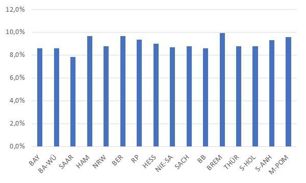
I. b) Accessibility by patients to PCR tests to generate confirmed cases

In Germany, only cases which were tested positive by a nationally normed PCR test are
counted as confirmed. Throughout the entire study period until 23 April, it was usually only
possible to become tested on prescription by a medical doctor. Only in a few rare instances
did local authorities arrange and allow selective mass testing of specific population groups.
This policy changed significantly from the end of April onwards, making tests available to
several general population groups on a precautionary basis, for instance professional soccer
players. However, during the study period, this was a rare exception.

Throughout February and in the first week of March, obtaining a test was difficult and
discouraging. Until then, most tests were conducted in hospitals, if treated patients were
suspected of being infected. Usually this meant having an exposure to China or, in the second
half of February to Italy. Both testing capacities in laboratories and testing facilities had not yet
been widely available, nor was there a clearly formulated testing strategy. Until 8 March only a
total of 124,716 tests had been conducted, with 3.1% positive results. The overwhelming
majority of those tests were conducted in the last week of February and first week of March.

During the second week of March up to 15 March, both testing capacity and accessibility
multiplied, and from 23 March onwards, the system-wide testing capacity was regularly twice
as high as the number of tests being performed. Until 15 March, a total of 348,619 tests were
conducted (6.8% positive), with 361,515 (8.7% positive) by 22 March, and 408,348 (9,0%
positive) by 29 March. During April the positive test rate declined by the week, from 8.1% to
6.7% to 5.0% to 3.8% by the end of April 6.

As explained in the main report, the statistical evidence suggests that in the course of April,
symptomatic persons increasingly avoided being tested, even though testing capacity was
amply available and free of charge to the patients. This may possibly be due to the perceived
“punishment” of imposition of self-isolation imposed by the public authorities if a household
member is tested positive, with no “reward” of any medical treatment which would improve the
medical conditions.

From 16 March onwards, the majority of tests were usually conducted at specially arranged
testing centers which were operated by either doctors or city councils in various formats. Most
were walk-in, while drive-thru centers remained rare. During the third and fourth week of
March, the number of tests conducted per weekday throughout Germany remained roughly
the same. However, the rate of positive results kept increasing from Monday to Friday. From
30 March onwards the opposite happened. While the number of tests was roughly the same
per weekday per week, the rate of positive results kept decreasing from Monday to Friday 7.
Hospitals tested on all seven days of the week.

During March, the testing strategy required patients to have typical covid-19 respiratory
symptoms AND to have one of four further conditions; a) either travelled to a high risk area, or
b) to having had close contact with a confirmed case, or c) being a high risk person, or d)
working in the medical or care sector. As the borders had been closed by the middle of March,
the travel condition became meaningless. Non-symptomatic or atypical (for instance not
respiratory) cases were generally not tested, unless they were hospitalized. Medical or care
personnel were never mass-tested as a rule. Whether this was a wise testing strategy has been
the subject of public debate, but for statistical purposes, it had the benefit of being consistently
applied throughout all of Germany and the entire study period up to 23 April 8.

                                             3   SI, S II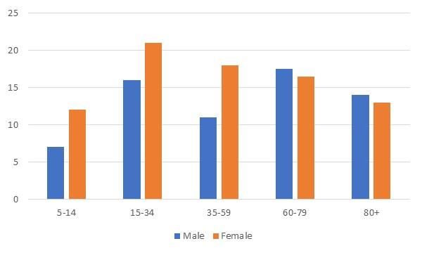
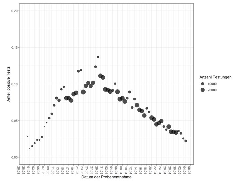
Figure S I a) PCR test statistics for Germany

Source: Robert Koch Institut Täglicher Lagebericht zur Coronavirus Krise 06 May 2020.

Headers: CW – number of tests – positive tests – number of laboratories

                                                  4    SI, S II
I. c) Official compilation process of the confirmed cases data
Data on positive test results have been compiled at two levels. Each county has a public health
office (Gesundheitsamt) which is in charge of local health monitoring. Doctors and hospitals in
this county report all their cases to this local health office, where they become registered on
the day of receipt of the report. The counties have had differing registration systems. Some
counties accepted cases for registration on the weekend while some did not, and some
changed from one status to the other over time. There may have also been bundling effects in
the transmission of data from the testing centers to the local health offices.
From the local offices, the data are reported to the federal agency in charge of coordinating
the covid-19 public health response, which is the Robert Koch Institute (RKI). RKI reports all
data which it receives per day, on its dashboard website the next days (the presentation day),
which is refreshed once during the night. The data is presented in various dimensions for the
national level, the state level and the county level. The first dimension is: “Daily new infections
as per the registration date at the local public health office (not the receipt date at RKI)”.
Because transmissions from the local offices may differ and because there are frequent
corrections, the data is assigned retroactively to the original local registration dates.
Corrections and additions still occur several weeks later. The second dimension is: “Date of
first symptoms when known, plus date of local registration for those where first symptoms are
not known”. This is a confusing picture, because there may be several days of delay between
symptoms and registration, so that two different categories of incidences are shown per day.
The third dimension is: “Cumulative age distribution of all cases until the presentation day”.
The age distribution is not shown for previous dates, but instead it is shown in absolute and
also per 100,000 inhabitants. The fourth dimension is: “Number of cumulative deaths until
presentation day”. During the study period up to 23 April, no data on negative test results were
reported, neither at the local nor the national level.
Since 16 April, RKI employs a Nowcasting method to estimate an “R” across the German
epidemic experience. Its methodology was explained in detail on 23 April 9. In its Nowcasting
model, the RKI takes the day of first symptoms as its key variable. For those cases for which
these are not known, the registration dates are imputed backwards with sociodemographic
estimates, according to a method described by Lawless in 1994 10. Data for recent days that
have not yet been fully registered and transmitted to RKI are being estimated by a similar
method. RKI does not publish the details of its model nor the regression coefficients it uses,
and also does not publish Nowcasts per state or county.
With its Nowcasting model, RKI shows that the peak of newly shown symptoms was reached
on Wednesday, 18 March in Germany. The Nowcast clearly shows that there are successive
small peaks on each following Wednesday, on 25 March, 01 April and 08 April. Given the by
now well-established incubation period of predominantly 5 days from infection to symptoms 11
12 13
, this is proof that Fridays were the most infectious days for the covid-19 epidemic.
Since the Nowcast of date of first symptoms is not available on a regional basis, this article
uses the local registration dates as reported by RKI on its presentation day, as the basis for all
calculations. This has the main disadvantage that these data inherit the weekend troughs when
neither the testing centers nor local offices were working. The weekend troughs may also
5 SI, S IIcontain a component of test discouragement by symptomatic people, who might have given
up on being tested if it was not possible on the weekend. Except for a few instances in cities in
the first weeks of March for the cases studies, when the registrations on a Monday obviously
represented a three-day count including the weekend, the analysis did not correct for those
weekend troughs.
Figure S I b) Nowcasting model of covid-19 epidemic in Germany, by RKI
Source: Robert Koch Institut Täglicher Lagebericht zur Coronavirus Krise 06 May 2020
Translation of subtext: Cases with known onset of symptoms (dark blue), estimated onset in cases with no onset
data (gray) and estimated progression of symptomatic cases (light blue); status 6 May 2020, 0.00 hrs, considering
cases up to 2 May 2020
I.d) Reporting intervals from infection to death
The raw data provided by RKI on its dashboard strongly suggests that there is a 14-day interval
between infection and local registration day. This interval seems to have been decreased to 10
days in the course of April.
The interval of 14 days are plausible on the observation that the mean incubation period
appears to be 5 days, and that it then took 9 days from onset of symptoms towards registration.
Those 9 days would split into time for the patient to make the decision to obtain a test, receiving
a testing date, transporting and processing the specimen in the laboratories and then remitting
a positive result to the local healthy agency. There would be additional time until the results
are presented by RKI. However, RKI would always retroactively assign the notice to the day of
the registration. It appears that in April the time from symptoms to registrations came down to
5 days.
The death interval from infection to reporting at RKI appears to be 28 days. This would split
into an incubation period of 5 days, average time to admission in a hospital 8 days, average
time to clinical deterioration and death of 10 days, and then reporting to RKI in 5 days. These
intervals are well supported by the international literature, but no specific intervals for Germany
6 SI, S IIcould be identified in publications. The death numbers are not retroactively assigned by RKI,
but are counted as per day of receipt of report.
Several case studies examined in Supplement V support the calculation of a reporting interval
of 14 days, where case registrations follow exactly 14 days after a known super-spreading
event. Another piece of evidence is that the death-incidence and age-adjusted factor (DAF
method, explained in Supplement II) which is employed in this analysis generates a peak of
90,000 newly registered infections on 27 March, nine days after the Nowcast peak of 18 March,
for a nine-day difference. Adding five days of incubation, this suggests that there was on
average across Germany a 14-day period between infection and registration at the local health
authority. This period is also corroborated with RKI data on the estimated data transmission
periods in its Nowcast methodology paper. This study therefore consistently assumes that
during March there is a 14-day period between infection and local registration as shown on
RKI presentation day.
Throughout the course of April, as testing became more widely available, and the testing
system had been well established, the period from infection to registration appears to have
shortened to around 10 days. This reduction was not included in the analysis of the DAF
method, but it is shown in the presentation of the data for the natural experiment comparison
between the German states in Section 3 of the main text. Shortening the infection to registration
period in April to 10 days, does not have a noticeable impact on the analysis, and changes
none of the observations and conclusions.
I. e) General socioeconomic controls in the county data
As a control for the analysis, a series of simple correlation tests were conducted among the
401 counties, in order to identify which factors were likely or unlikely to have influenced the
transmission dynamics of the epidemic. The German counties differ in several socioeconomic
dimensions, which may have had an impact. If so, this should be visible in the data. Detailed
socioeconomic data for the counties are available from the German census data from 2011.
The five variables tested were: 1) rural vs urban using an index published by the German
Ministry of Agriculture 14; 2) taxable income 15; 3) population density ; 4) housing conditions
and 5) household composition 16. The first three did not show significant correlation effects,
with neither sufficient t-values nor p-values, neither on their own, nor as a multivariate analysis.
Especially the first factor seems surprising, because a casual look at the map of Germany would
suggest that rural counties are more affected by covid-19 than the cities. However, statistical
analysis on a county level refutes this hypothesis. Likewise, the experience from other
countries, especially Spain, France and United Kingdom would have suggested that dense
urban centers should be more heavily affected. This too can be refuted, at least for the German
experience.
As for housing conditions, the census data provides various details, such as vintage year of
building, ownership types of buildings, types of heating, number of living units per building,
type of building, and size of living units. Most of these variables did not generate meaningful
correlations which survive deeper scrutiny. Notable exceptions were only size of living unit of
80-99 sqm, where those counties with proportionately more of these units were positively
correlated with higher infection rates at 32% (t-value 6.8), a housing stock built between 1991
and 1995 being correlated with 39% (t-value 8.3), and buildings with two living units being
correlated at 33% (t-value 7.0). A causal explanation cannot be provided for these correlations,
7 SI, S IIand requires separate investigation. At any rate, 81% of the German housing stock is older
than 30 years. So there could not be a connection of potential dilapidation of housing stock
and infection rates per county.
Household composition yields a clearer picture of correlations for which an explanatory
hypothesis can be formed. Counties with proportionately more households consisting of
couples with children are positively correlated to higher infection rates by 28% (t-value 5.9);
counties with more couples without children are negatively correlated by -34% (t-value -7.3).
Having more single person households is also negatively correlated by -12% (t-value -2.4), but
less important than the household criteria with or without children. Single parents or shared
living households have no significant correlation. When focusing only on families, then married
couples are positively correlated by 26% (t-value 5.4), and unmarried couples are negatively
correlated by -27% (t-value of -5.7). When focusing on the size of the family, then four or five
persons in the family are highly correlated by 44% (t-value of 9.6). Two or three persons in the
family are negatively correlated at -39 and -5% (t-values of -8.4 and -1.1) respectively. Finally,
having a senior citizen in the household is correlated with 19% (t-value 3.9).
The theme which likely emerges from these household composition correlations is that
counties with a higher share of what might be called traditional family structures, with married
mother and father and several children plus possibly a grandparent as well, experienced
significantly higher rates of infection, than counties with relatively more of non-traditional types
of living arrangements, such as unmarried couples, single parents or single households. The
difference are not the children, because unmarried couples with children and single parents
are also negatively correlated. The difference thus appears to be traditional versus non-
traditional. The hypothesis is that counties with more traditional family structures also maintain
a stronger social network with more points of interactions within the private sphere, so that this
private sphere created a larger close-contact reservoir for infection chains. Further research
needs to corroborate this hypothesis.
Figure S I c) Co-variate analysis of three key socioeconomic variables
Regressions-Statistik
Multipler Korrelationskoeffizient
0,19226403
Bestimmtheitsmaß
0,03696546
Adjustiertes Bestimmtheitsmaß
0,02696856
Standardfehler 150,35326
Beobachtungen 293
ANOVA
Freiheitsgrade
Quadratsummen
(df) Mittlere(SS)
Quadratsumme
Prüfgröße
(MS) (F) F krit
Regression 3 250771,256 83590,4187 3,69769259 0,01225523
Residue 289 6533163,7 22606,1028
Gesamt 292 6783934,96
KoeffizientenStandardfehler t-Statistik P-Wert Untere 95% Obere 95% Untere 95,0% Obere 95,0%
Schnittpunkt -11,912717 93,7529089 -0,127065 0,89897729 -196,4378 172,612362 -196,4378 172,612362
Density -0,0158294 0,03435109 -0,4608107 0,64528099 -0,0834394 0,05178069 -0,0834394 0,05178069
Ländlichkeit 22,7149789 25,4591309 0,89221345 0,37302081 -27,393846 72,8238042 -27,393846 72,8238042
Einkünfte 0,07713581 0,03041711 2,53593515 0,01174154 0,01726867 0,13700296 0,01726867 0,13700296
Source: Own calculations for this article
8 SI, S III. f) Additional background to the six bundles of social distancing mentioned in Section 3
In addition to the short descriptions of each bundle of social distancing mentioned in Section
3 of the main report, the following provides more context and color to each of the bundles
1) Context to the first bundle, the end of carnival and winter vacation season, 03-06 March
Traditionally, the week after carnival, which was celebrated in 2020 from Saturday 22 to
Tuesday 25 February, is the second busiest winter vacation week in Germany. Three million
Germans will travel to the Alps during this week, which is almost as much as in the first week
of January, and five times as much as during any of the other winter weeks 17.
The five most engaged states in winter sports are Bavaria, Baden Wuerttemberg, Berlin, Hesse
and North Rhine-Westphalia, at roughly twice the engagement rate of the other states. Of these,
three had a school vacation from 22-29 February, which were Bavaria, Baden Wuerttemberg
and North Rhine-Westphalia. The latter two are also highly engaged in the carnival celebrations,
which shows itself in Section 3, Figure 6 with increasing Rta values on carnival weekend of 22-
24 February. All three of them including Bavaria, show increasing and high Rta values on
Friday/Saturday 28/29 February. This Saturday would have been the day when one-week-long
vacationers were ending their vacations. After that the Rta of these three states rapidly drops
for several days in a row.
A second group of states (Hamburg, Rhineland-Palatinate, Hesse and Lower-Saxony) see the
maximum of their R at around Monday, 02 March, before abruptly declining for several days.
As these states do not have school vacations in the carnival period, their Rta numbers are likely
dominated by people without school children returning from extended weekend stays in the
Alps. By the end of the week on Sunday 08 March, their Rta had dropped from around 3 to 1.
A third group of states without winter vacation lifestyles (Saarland, Berlin, Saxony,
Brandenburg, Thueringen, Schleswig-Holstein and Mecklenburg-Vorpommern) sees only a
gradual and moderate reduction of their Rta across the first week of March (whereby Bremen
and Saxony-Anhalt are outliers). Its Rta’s stood at around 1.5 at the end of the same week,
though the group had a low level of prevalence, as there were almost no infections throughout
February, and only little exposure to the infectious Alps.
2) Context to the second bundle, voluntary social distancing behavior, 07-10 March
Besides the media coverage and deteriorating macroeconomic situation explained in the main
text, there was also an extensive public media discussion in Germany on whether large scale
events should be banned or not, in particular whether it was feasible to continue the national
soccer league and public attendance of its matches. The discussion was reinforced by the
decision of the Italian government to impose quarantine on all of Italy on 09 March, and driven
by a number of high-profile infections of senior politicians and celebrities. By the end of Monday
09 March, even without a national policy declaration, regional authorities everywhere had
banned all scheduled large festival events, sports events and trade fairs. This was followed on
the Tuesday with a national government recommendation not to conduct events with more
than 1000 participants. At first the soccer leagues intended to continue playing in empty
stadiums, but by Friday 13 March all games were cancelled until further notice.
9 SI, S IIThe de facto national ban on large-scale events effectively applied only to the events of the
following weekend onwards, because it was declared after the weekend on Monday 09 March.
The effectiveness of this public policy measure to ban events of more than 1000 people cannot
be directly assessed, because there were no states which allowed such events, so no
differences can be observed.
The effectiveness of this second bundle of voluntary behaviors also profited from the natural
end of the winter vacation season one week before, because that stopped the fresh imports of
super-spreading activity in the Alps. The important exception is Bavaria where winter sports
continued, so this difference can be observed. The residents of Southern Bavaria continued
to visit the Alps, as is shown in the case studies in Supplement V, and therefore a large part of
the state kept on importing cases from super-spreading activity. The Bavarian Rta had only
reached a value of 2 on the weekend of 07/08 March, and dropped to 1.4 by the middle of the
following week, while other large winter-vacationing states such as Hamburg or North Rhine-
Westphalia had already reached 0.6. The difference between an Rta of 1.4 and 0.6 can be
assigned to the continuation of exposure to the super-spreading activity in the Alps.
3) No further context to the third bundle
4) Context to the fourth bundle, mandatory social distancing of contact bans, 23-26 March
During the third week of 16–20 March, the German national government lost some control over
the virus agenda. As PCR tests became more widely available, the number of newly confirmed
cases was skyrocketing. In parallel, coverage of the corona crisis by the media escalated even
faster. Video coverage and eye-witness stories from Italian hospitals became more alarming
by the hour. Germany suddenly found itself surrounded by countries that imposed much
stricter social distancing measures. In both Austria and France, citizens were not allowed to
leave their homes unless for necessary reasons which needed to be proven in writing and they
were not allowed to meet members of other households. While in Germany restaurants were
still open, Switzerland closed all restaurants on 17 March. As per 20 March the Swiss
government also banned all gatherings of more than 5 people in public spaces, while in
Germany there was no policy mandate on keeping distances or group sizes. Scientific experts
and the media were suggesting in a growing chorus that Germany was not doing enough to
contain the epidemic.
The Apple mobility data also clearly show the national differences as well (but did not become
available until 14 April, so were not yet known at that time). By Friday 20 March, German
walking had reduced to 45%. By comparison, the Austrians were down to 32%, the French to
16%, Italians down to 17% and Spanish were below 10% of their normal level of walking. Only
the Danes were more mobile than the Germans at 55% walking (the Danes’ lowest value was
reached on 18 March at 46%).
Under public pressure the government of Bavaria suddenly decided without warning or
coordination to impose an Austrian-style lockdown on its population on Friday 20 March. The
prime minister of Bavaria was applauded for this step in the media, and so the other German
states felt compelled to follow. As a response, over the weekend, the national government
decided to launch its second bundle of MSD, which went into force from Monday 23 March
onwards 18.
10 SI, S II5) Context to the fifth bundle, the first summer-like weekend, 03-07 April
As the epidemic unfolded further over the weeks after the MSD of contact-bans were enacted,
public debate moved on. On the one hand, the world began to look admiringly at Germany for
its low case fatality rate. It also became obvious that Germany had significantly more ICU beds
than it would need. The health care system was actually idling, because all non-urgent
procedures had been cancelled or postponed, while the surge of covid-19 patients failed to
arrive. On the other hand, while it became clear that Germany had avoided a medical
catastrophe, the economic costs of the crisis began to surface. The automotive industries,
which are Germany’s largest industrial sector, had shut down for lack of demand and disrupted
supply chains; the transportation sector was a shadow of itself; freelancers of all stripes in the
gig economy had lost much of their income, not to mention those businesses which were
forced to close, such as personal services, retailing, entertainment, trade fairs and others. The
public debate began to shift towards how to exit from shut-downs and contact-bans, and
whether they had been such a wise choice to begin with, on economic grounds.
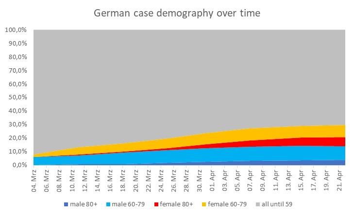
In the midst of this debate, April began with the first summer-like temperatures of the year.
The official explanation by the Robert Koch Institute for the rise of its own calculated R value
during this period, was that more senior citizen homes had become infected, and therefore a
rise in infection rates as well as mortality should be expected. This claim was factually not true.
Indeed, the case demography had grown steadily older throughout March, but around the
beginning of April that trend began to actually level off.
Figure S I d) Changes in the case demography over time
Source: Own calculations for this article
11 SI, S IISupplement II
Additional Details on Calculation Methods Used
Subjects:
a) Background
b) The DAF Method and the Gangelt IFR
c) Excess mortality considerations
II. a) Background
Throughout March, the president of RKI, Lothar Wieler suggested implausibly and without
factual evidence that the reported confirmed cases represented relatively closely the actual
progression of the epidemic, and that the number of hidden cases “was not very high” 19.
However, at no point were representative mass tests undertaken in Germany, to provide an
estimate of the hidden case number, or for corroboration of the federal agency’s assumption.
In April, RKI promised to conduct antibody tests in order to obtain a better estimate of the real
infection status versus the confirmed case numbers. No such results were yet made available
in the course of April. As in other countries, the antibody tests available in April had suffered
from a lack of sufficient specificity, so that testing in low prevalence environments generates
too many false positive 20. As a result of the conviction that the confirmed case numbers closely
mirror the actual epidemic, the official R numbers published by RKI are based on confirmed
case numbers only. No attempt was ever undertaken to estimate the size of hidden numbers
and to incorporate this into the officially published R.
However, in various locations around the world, including German Heinsberg, in Austria, Spain,
California, New York and more, such investigations into the real scale of infections yielded
substantial hidden case numbers, with factors 5 to 50 21 of the actually confirmed cases. In mid-
March, Mizumoto et al estimated an infection fatality ratio (IFR) for Wuhan of 0.12% 22, while
Verity et al estimated a 0.66% for China 23, which became the basis for various publications by
the Imperial College London. These two estimates also imply several multiples of hidden case
numbers versus confirmed case numbers.
As of writing this article, the so far only in-depth investigation for an IFR in Germany explored
the case study of the Gangelt carnival outbreak in the county of Heinsberg with a representative
sample of 919 persons in 405 households out of a city of 12,597 inhabitants. It yielded an IFR
of 0.41% 24. This is the value which is utilized in this study as the general IFR. The U.S. CDC is
using 0.4% in its estimations as per end of April.
II. b) The DAF Method and the Gangelt IFR
For estimating the real rates of infections throughout all German states and counties and using
them to assess the effectiveness of social distancing measures, the analysis follows an adapted
method to Flaxman et al. from ICL’s Report #13 25. The analysis uses the Gangelt IFR as a base
number to calculate corresponding real case numbers for each of the German states. The
starting assumption is that the implied infection fatality ratios (IFR) per age group in Heinsberg
12 SI, S IIare the same across all Germany, and also are the same across the entire progression of the
epidemic until April. There are no reasons to assume otherwise, since the German health care
provision system is identical throughout the country. Furthermore, at no point throughout
March or April did the German system experience a breakdown, nor did the county of
Heinsberg experience a breakdown of its system, so that no local effects should exist. There
were also no new medications or treatment protocols arriving during this period which would
improve the clinical outcomes of the disease.
It should also be noted that for the purposes of this article, it is not relevant to what degree the
IFR of Heinsberg misestimates the IFR for all of Germany. Ultimately, this IFR represents only
a multiplication factor for all other subsequent calculations. If the IFR is higher or lower, this
only increases or decreases the factor, but it does not change the relationships between the
different dynamics of the epidemic between the states. It only changes the estimate of absolute
total number of infected, but is of no substantial consequence to the reproduction number Rta
that are derived from it.
While the age-adjusted IFR are assumed to be the same across place and time in Germany,
the different states did experience different attack rates in their age groups, as implied by their
respectively different demographics of the cumulative confirmed cases (CCC) load. Also, the
age groups were differently attacked throughout the progression from March to April. At the
beginning, Germany registered only few senior citizens among its cases, but over time the
older age groups became more prevalent among the CCC.
One of the surprising outcomes of the Gangelt-Heinsberg investigations is that the rate of
infection was rather similar across all age groups, from teenager to the very old, namely around
15%. Out of the 12,597 inhabitants and their extrapolated 1,955 infected persons, 8 persons
died of covid-19 until the study period in mid-April, making for the IFR of 0,41%. However,
those 8 persons do not permit the calculation of an age-specific fatality ratio. The assumption
is that the IFR for the city of Gangelt is applicable to the German average demographic
composition of infections as per 22 April, so about three weeks later. The justification for this
shift is that the Gangelt outbreak occurred about three weeks before the explosion of the
epidemic across Germany.
Figure S II a) Real infection rates in Gangelt case study participants, in%
Source: Streeck et al. University of Bonn, Heinsberg case study
13 SI, S IIThe analysis in this article conducts the following calculations
a) From RKI this analysis scrapes the demographic composition of all deaths that were
reported to it until Tuesday 05 May, and published in its daily bulletin on 06 May. This
composition is provided by male/female and in five age groups of below 60, 60-69, 70-
79, 80-89 and above 90. RKI also provides the demographic composition of the CCC
load as reported to it until Tuesday 21 April, and presented on 22 April. To any degree
that some counties may take longer than others to transmit their data to RKI, their
respective numbers would be missing in both totals. On the assumption that there is an
average of 14 days between local health agency registration of case infections until
death (see Supplement I d), then it is the CCC load presented on 22 April that generated
the cumulative deaths presented on 06 May. From this data, the analysis proceeds to
calculate five specific 14-day time-delayed age group case fatality ratios (TDCFRage):
for men above 80, for women above 80, for men between 60 to 79, for women between
60-79, and for all others. Note, that different assumptions on the time period between
local registration and presentation of death at RKI would only change the multiplication
factor for the remainder of the analysis, but would not change the comparison dynamic
between the states.
b) RKI is providing the same demographic composition of CCC load also for each state
and for each county, but the demographics of deaths is only provided on a national
level. In the analysis, the assumption is made that the TDCFRage is the same across all
of Germany and all across all March and April. There are no systematic reasons to
believe otherwise.
c) Each state has a different demographic composition of its CCC, which likely reflects
different attack rates on the age groups per state or county. So a state with an older
CCC, is likely to incur more deaths, for which the calculation needs to be adjusted. With
standard arithmetic, the data are adjusted towards the overall German composition, to
calculate how many deaths the states or counties would have incurred, if they had had
the national German demographic composition of CCC. This number is then divided by
the Gangelt IFR to yield the cumulative real cases (CRC) of infections which must have
occurred in each state until April 22. For instance, the state of Berlin reported 159
deaths until 06 May, but because it has a younger CCC than Germany overall, these
deaths represent a proportionately larger group of CRC of infections, on the assumption
that the younger CCC also represents relatively more attacks on the young in Berlin.
The nationally adjusted number of deaths Berlin would have had is 229. Dividing those
229 by the Gangelt IFR yields 56,062 cumulative real cases (CRC). Dividing the
reported number of deaths by the CRC provides the IFR state per state, which in the
case of Berlin is 0.28%.
d) Dividing the CCC load by the CRC load, provides a state-specific cumulative death
incidence and age-adjusted identification rate (CDAIRstate) of cases as per 22 April.
Figure S II b) shows that this CDAIR is similar across all states, which confirms that the
testing strategy was more or less the same across all states. The German average
CDAIR was 8.8%. For instance, the Berlin CCC until 22 April was 5,410, which divided
by 56,062 real cases gives a Berlin CDAIR of 9.7%
e) Then the analysis calculated the CDAIR for each week beginning from the first week of
March for all of Germany. For each week, an estimate was made of deaths to be
expected, given the CCC load and the respective demographic composition until that
week. For instance, the CCC load of 31 March, given its demographic composition,
14 SI, S IIshould have generated 2,618 deaths two weeks later on 15 April. However, there were
actually 3,255 deaths recorded on 15 April. This means that the CDAIRweek until 31
March was by a factor of 1.24 lower than on 07 April, or actually 7.1% instead of 8.8%.
Counting the four previous weeks in reverse order, the CDAIRweek dropped to 5.3%,
3.7%, 2.4% and 1.9% respectively. This CDAIRweek was then interpolated for each day,
so that daily CDAIRdaily became available from Monday 02 March to 22 April.
f) The newly confirmed cases (NCC) of each day of each state were then divided by these
CDAIRdaily and adjusted to the CDAIRstate of each state to arrive at the newly real case
(NRC) load of each day in each state. This calculation assumes that the respective case
demographies grew older at the same rate in each state as in Germany overall. This is
almost certainly not the case, but the potential error is only of marginal significance at
the level of state aggregation.
g) All new cases were summed up per day across all states, and compared to the actually
registered number of cases per day on country aggregation level. This provides a daily
death-incidence and age-adjusted factor (DAF) by which the reported NCC are lower
than the NRC (Figure S II c). Straightforward division also reveals the daily current IFR
which is always higher than the cumulative IFR, as long as the case demography keeps
aging (Figure S II d).
h) For the case studies on county level, the daily NCC were multiplied with the daily DAF,
in order to arrive at the county specific new real cases NRCcounty per day, which could
then easily be summed up to the CRC. The NRCcounty were not calibrated for a county-
specific CDAIR or their case demographies, even though these tended to vary a lot on
state level. Several counties CDAIR are only half of their states, suggesting that locally
the national testing strategies were either differently implemented or the cases were
more difficult to identify. This calculatory simplification was justified as it did not impact
the learnings from the case studies on county level. Where large differences exist, they
are mentioned in the case study.
Figure S II b) Cumulative death-incidence and age-adjusted identification rate (CDAIR)
How to read this chart: Cumulatively until 22 April, 9.7% of all cases were identified in Berlin
Source: Own calculations
15 SI, S IIFigure S II c) Death-incidence and age-adjusted factor (DAF)
50
45
40
35
30
25
20
15
10
5
-
11.03.2020
21.03.2020
31.03.2020
09.03.2020
13.03.2020
15.03.2020
17.03.2020
19.03.2020
23.03.2020
25.03.2020
27.03.2020
29.03.2020
02.04.2020
04.04.2020
06.04.2020
08.04.2020
10.04.2020
12.04.2020
14.04.2020
16.04.2020
18.04.2020
20.04.2020
22.04.2020
How to read this chart: On 12 April, one out of five real cases became known as a confirmed case
Source: Own calculations
Figure S II d) Daily current infection fatality rate
How to read this chart: On 22 April, the reported number of deaths represented 0.82% of the real cases that became
infected 28 days earlier on 25 March, and were partially identified (at the CDAIR) 14 days earlier on 07 April. The
rising rate indicates that the case demography grew older over time.
Source: Own calculations
16 SI, S IIII. c) Excess mortality considerations
In addition to the hidden number of cases, there is also a hidden number of deaths. These can
be estimated from excess mortality. On 30 April, the German federal statistics agency provided
a special report on mortality experienced by each state until 05 April 26. A difference-in-
differences analysis shows that there was significant excess mortality starting from the middle
of February onwards, however, not to the same degree in all states. Besides Austria, Germany
was the only other country in Europe to experience excess mortality from the middle of
February forward. The state of Bavaria experienced excess mortality already from the middle
of January onwards, implying that there was considerable infection activity at latest from the
beginning of January 2020 onwards.
Until 05 April, there were 2,503 deaths too many in Germany (out of a total of 269,943),
compared to what would have been expected given the trend in the beginning of 2020, in
comparison to the previous five years (which includes the strong influenza season of 2018). Of
these deaths, 1,342 can be attributed for by covid-19, which leaves 1,161 deaths that are
unexplained. It cannot be known whether these are deaths that are directly caused by covid-
19 but which were undetected, or whether these are deaths which were indirectly caused by
covid-19, for instance heart attacks or strokes that went untreated because the patients were
reluctant to visit the doctor or the hospital during the covid-19 crisis, or because there was a
third unknown cause. The second reason should not have been the case, because Germany
had sufficient hospital capacity throughout the entire crisis, but it is possible.
In contrast to many other countries, Germany has had a policy of not testing diseased persons
for covid-19, so it is most likely that the large majority of unexplained deaths are persons who
died at home because of covid-19, without being diagnosed for the disease.
Out of the unexplained deaths, 1,008 or 87% were accumulated in only three states, Bavaria,
Baden-Wuerttemberg and North Rhine-Westphalia, which also are the states which were
affected earliest and most seriously by the epidemic. However, there is no correlation between
level of infectedness and unexplained deaths among the other 13 states.
Of the unexplained deaths, 399 occurred before 15 March, of which 369 or 92% occurred in
Bavaria, Baden-Wuerttemberg and North Rhine-Westphalia. Officially there had been only 15
deaths from covid-19 until that day, all of them in these three states. Given the four-week delay
between infection and reporting, all of these 399 deaths represent infection activity in Germany
before and until 16 February, which means they occurred even before the first known super-
spreading event of Gangelt in Heinsberg on 15 February.
All of the above considerations compare excess mortality against the average of the previous
five years, which systematically underestimates the covid-19 related mortality because the
strong influenza season of 2018 is included. The calculations in Section 3 of the main report
delves deeper into the numbers and compares the excess mortality against the more typical
mild seasons only, and also compares them on a trend basis, which yields more accurate
results.
One question is, how this excess mortality should be and can be computed into the IFR (see
previous section Supplement II b). According to Streeck et al., there was no excess mortality
in Gangelt besides the 8 recorded cases due to covid-19.
Dividing the unaccounted for 1161 deaths with the IFR of 0.41% yields a total number of
283,170 additional infections until 08 March.
17 SI, S IIDividing the 399 – 15 = 384 deaths until 15 March, with the IFR of 0.41%, yields a total number
of infected persons of 93,658, who were infected in these three states from before and up to
16 February – if the expected mortality is conservatively assumed to be the average of the
previous five years (actually the expected mortality should be oriented at the year 2016 only,
which had a similarly mild influenza season as 2020).
This would indicate that the total number of infected persons must be even higher than what
is implied by the known number of deaths, and that the above roughly 283,000 additionally
infected persons should be added to the total of 1.84 million cases as per 30 April (the 1.84
million are calculated by the DAF method. They are roughly equivalent to the 7724 official
deaths as of 14 May, divided by the IFR of 0.41%). However, the earlier IFR were likely to be
lower because the attack rates on the vulnerable old age groups appear to have been lower
during the early phase of the epidemic (at least as indicated by the lower confirmed cases).
So, it might have been an additional 500,000 infected persons who need to be added to the
total, to account for January and February infection activity.
It is also possible to speculate that the ratio of unaccounted excess mortality would have
continued throughout April, in which case the entire overall number of infections would need
to be nearly doubled to about 3.4 million by the end of April. This would mean an overall
infection rate of about 4% of the German population. The nationwide serological sample
conducted by the Spanish authorities with 60,000 tests, results in an overall infection rate for
Spain of around 5% as of 13 May 27. Therefore 4% for Germany may be a reasonable estimate.
The other direction of thinking would be to assume that the hidden number of deaths resulted
from the same pool of infections, and that in reality it is the IFR which needs to be adjusted
upwards from 0.41% to 0.76%.
None of this can be concluded without more data becoming available over the next few weeks
and months. It is also not particularly relevant to the assessment of social distancing
effectiveness, because it ultimately only changes the multiplication factor. It would only make
a big difference if the CDAIR, the identification rate, would have rapidly increased in April over
March. But if anything, the evidence points to the contrary, that the CDAIR decreased.
18 SI, S II1
https://www.eurosurveillance.org/content/10.2807/1560-7917.ES.2020.25.9.2000178
2
https://www.zeit.de/wissen/2020-04/coronavirus-intensivbetten-deutschland-auslastung-kapazitaeten-
tagesaktuelle-karte
3
https://ourworldindata.org/covid-testing
4
Daily Bulletin of Robert Koch Institut from 22 April 2020
https://www.rki.de/DE/Content/InfAZ/N/Neuartiges_Coronavirus/Situationsberichte/2020-04-22-
de.pdf?__blob=publicationFile
5
https://npgeo-corona-npgeo-de.hub.arcgis.com/
6
Daily Bulletin of Robert Koch Institut from 06 May 2020
https://www.rki.de/DE/Content/InfAZ/N/Neuartiges_Coronavirus/Situationsberichte/2020-05-06-
de.pdf?__blob=publicationFile
7
Daily Bulletin of Robert Koch Institut from 22 April 2020
https://www.rki.de/DE/Content/InfAZ/N/Neuartiges_Coronavirus/Situationsberichte/2020-04-22-
de.pdf?__blob=publicationFile
8
https://www.welt.de/wirtschaft/article207572591/Corona-Diagnostik-Bundesregierung-rueckt-von-
Massentests-ab.html
9
Epidemiological Bulletin 17/2020 from 23 April 2020
https://www.rki.de/DE/Content/Infekt/EpidBull/Archiv/2020/Ausgaben/17_20.pdf?__blob=publicationFile
10
Lawless J: Adjustments for reporting delays and the prediction of occurred but not reported events. Canadian
Journal of Statistics 1994;22(1):15 –31
11
Linton NM, Kobayashi T, Yang Y, et al. Epidemiological characteristics of novel coronavirus infection: A
statistical analysis of publicly available case data.
https://www.medrxiv.org/content/medrxiv/early/2020/01/28/2020.01.26.20018754.full.pdf
12
Sanche S, Lin YT, Xu C, Romero-Severson E, Hengartner N, Ke R. High contagiousness and rapid spread of
severe acute respiratory syndrome coronavirus 2. Emerg Infect Dis. 2020 Jul
https://doi.org/10.3201/eid2607.200282
13
Cheng H, Jian S, Liu D, et al. Contact Tracing Assessment of COVID-19 Transmission Dynamics in Taiwan and
Risk at Different Exposure Periods Before and After Symptom Onset. JAMA Intern Med. Published online May
01, 2020.
https://jamanetwork.com/journals/jamainternalmedicine/fullarticle/2765641?utm_campaign=articlePDF%26u
tm_medium%3darticlePDFlink%26utm_source%3darticlePDF%26utm_content%3djamainternmed.2020.2020
doi:10.1001/jamainternmed.2020.2020
14
Landatlas (www.landatlas.de). Ausgabe 2018. Hrsg.: Thünen-Institut für Ländliche Räume - Braunschweig
2018. © Thünen-Institut 2018
https://www.landatlas.de/wirtschaft/bip.html
15
https://www.landatlas.de/daten.html
16
https://www.zensus2011.de/DE/Home/Aktuelles/DemografischeGrunddaten.html?nn=3065474#Gitter
19 SI, S II17
https://wepowder.com/de/forum/topic/254948
18
Official website of the German government with the press release on Sunday 22 March specifying the social
distancing bundle of contact-bans:
https://www.bundesregierung.de/breg-de/themen/coronavirus/besprechung-der-bundeskanzlerin-mit-den-
regierungschefinnen-und-regierungschefs-der-laender-1733248
19
Geman Federal government press conference on 11 March 2020
https://www.youtube.com/watch?v=kPGT9pFIu8k&t=2833s
https://www.t-online.de/nachrichten/panorama/id_87542198/coronavirus-in-deutschland-wie-gross-ist-die-
dunkelziffer-.html
20
https://coronavirus.medium.com/a-99-accurate-antibody-test-8e404339f29a
21
https://www.deutschlandfunk.de/covid-19-wie-hoch-die-dunkelziffer-bei-den-
coronavirus.1939.de.html?drn:news_id=1124181
22
Early epidemiological assessment of the transmission potential and virulence of coronavirus disease 2019
(COVID-19) in Wuhan City: China, January-February, 2020; Kenji Mizumoto, Katsushi Kagaya, Gerardo Chowell
https://doi.org/10.1101/2020.02.12.20022434
23
Verity, R. et al. Estimates of the severity of COVID-19 disease. Lancet Infect Dis in press, (2020)
https://doi.org/10.1016/S1473-3099(20)30243-7
https://doi.org/10.1101/2020.03.09.20033357
24
Hendrik Streeck et al: Infection fatality rate of SARS-CoV-2 infection in a German
community with a super-spreading event, University of Bonn in May 2020
https://www.ukbonn.de/C12582D3002FD21D/vwLookupDownloads/Streeck_et_al_Infection_fatality_rate_of_
SARS_CoV_2_infection2.pdf/%24FILE/Streeck_et_al_Infection_fatality_rate_of_SARS_CoV_2_infection2.pdf
25
Seth Flaxman, Swapnil Mishra, Axel Gandy et al. Estimating the number of infections and the impact of non-
pharmaceutical interventions on COVID-19 in 11 European countries. Imperial College London (30-03-2020),
https://doi.org/10.25561/77731
26
Sterbefälle - Fallzahlen nach Tagen, Wochen, Monaten, Altersgruppen und Bundesländern für Deutschland
2016 – 2020:
https://www.destatis.de/DE/Themen/Gesellschaft-Umwelt/Bevoelkerung/Sterbefaelle-
Lebenserwartung/Tabellen/sonderauswertung-sterbefaelle.html
27
http://cadenaser00.epimg.net/descargables/2020/05/13/749ec6d73a8a14c1ed389711079cbfe5.pdf
20 SI, S IIYou can also read