Supplement of Quantifying the contributions of riverine vs. oceanic nitrogen to hypoxia in the East China Sea - Biogeosciences
←
→
Page content transcription
If your browser does not render page correctly, please read the page content below
Supplement of Biogeosciences, 17, 2701–2714, 2020
https://doi.org/10.5194/bg-17-2701-2020-supplement
© Author(s) 2020. This work is distributed under
the Creative Commons Attribution 4.0 License.

Supplement of
Quantifying the contributions of riverine vs. oceanic nitrogen to
hypoxia in the East China Sea
Fabian Große et al.

Correspondence to: Fabian Große (fabian.grosse@dal.ca)

The copyright of individual parts of the supplement might differ from the CC BY 4.0 License.
Große et al.: Hypoxia in the East China Sea–Supplement 1
S1 River input locations North of 31 ◦ N, the southward Yellow Sea Coastal Current
(YSCC) is simulated in summer and winter (Figs. S1a and b,
respectively), but it is weaker and reaches less far south in
Table S1. Center coordinates of input grid cells of all rivers con- summer. This behavior is within the range of existing mod- 35
sidered in this study and their associated nitrogen source groups. eling studies, which either simulate a consistent northward
‘None’ in last column indicates nitrogen from the river was not current (Bian et al., 2013) or a seasonal reversal of the YSCC
explicitly labeled as the river is outside of the tracing region (see (Guo et al., 2006). Existing observations are inconclusive on
Fig. 1, main text). the seasonality of the YSCC (Bian et al., 2013).
The surface inflow through Taiwan Strait is significantly 40
River name Latitude (◦ N) Longitude (◦ E) Source group lower in winter than in summer (compare Figs. S1a and c),
Liaohe 40.83 121.75 None due to the southwestward flowing East China Sea Coastal
Yalujiang 39.75 124.25 None Current with velocities of 0.1–0.3 m s−1 , which is in line
Luanhe 39.42 119.33 None with Bian et al. (2013).
Haihe 39.00 117.83 None The subsurface Kuroshio intrusion northeast of Taiwan is 45
Yellow River 37.58 119.08 None also present in winter (Fig. S1d), but reaches less far north
Hanjiang 37.42 126.42 None than during summer. A relatively strong westward current
Huaihe 34.00 120.42 None (up to 0.4 m s−1 ) at 125 ◦ E, 31–32 ◦ N originating from the
Changjiang 31.67 121.08 Changjiang Kuroshio is simulated in winter in both the surface and the
Qiantangjiang 30.25 120.92 Other rivers subsurface (Figs. S1c, d). This is in agreement with model 50
Oujiang 27.83 120.92 Other rivers
results of Guo et al. (2006), despite slightly higher current
Minjiang 26.00 119.75 Other rivers
velocities in our model.
In summary, our model agrees well with existing literature
with respect to the seasonality of surface and subsurface cur-
rents in the ECS. Thus, it provides a reliable basis for the 55
S2 Simulated circulation in the East China Sea source-specific nitrogen tracing.
Zhang et al. (in review, 2019) assessed the skill of the ap-
plied ROMS model with respect to the physics based on S3 Spatial patterns of dissolved inorganic nitrogen
5 sea surface temperature and salinity, which provides a ba-
A good representation of the spatial gradients and temporal
sic validation of the simulated hydrography. However, our
variability of nitrogen (N) concentrations in the ECS is im-
study of the contributions of the different nutrient sources
portant for reliable results of the N tracing applied in this 60
on hypoxia also requires a good representation of the gen-
study. Therefore, Figures S2 and S3 show spatial distribu-
eral circulation in the East China Sea (ECS). This is partic-
tions of simulated and observed concentrations of dissolved
10 ularly important considering the distinct seasonality of the
inorganic nitrogen (DIN; nitrate + nitrite + ammonium) in
region due to the East Asian monsoon. Furthermore, it is im-
the surface and bottom layers of the East China Sea off the
portant to evaluate simulated surface and subsurface currents
Changjiang estuary. The observational data were collected 65
as intrusion from the Kuroshio occur mainly in the subsur-
during nine individual cruises in 2010, 2011 and 2012 (for
face (Zhou et al., 2017a, 2018). Therefore, Fig. S1 shows
details see Gao et al. (2015)). The simulated DIN concentra-
15 average ocean current velocities and directions in the sur-
tions are averaged over the individual survey periods.
face (0–25 m; panels a, b) and subsurface ocean (25–200 m;
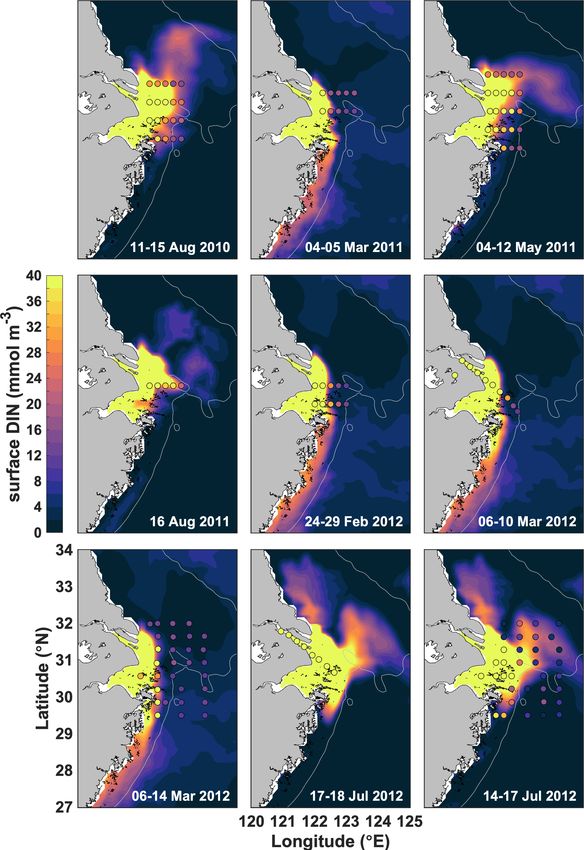
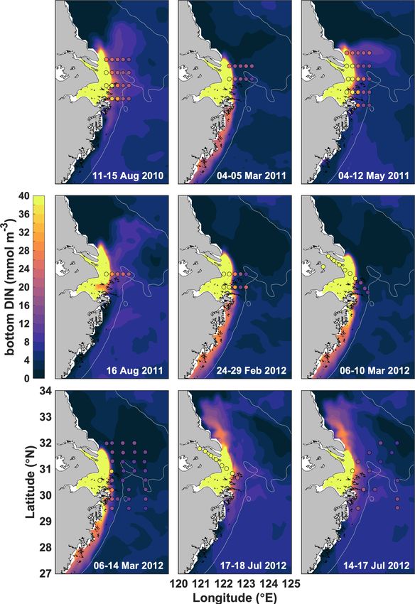
The model reproduces the general spatial patterns of DIN
panels c, d) during summer (June to August, ‘JJA’; panels
both at the surface (Fig. S2) and at the bottom (Fig. S3), espe- 70
a, c) and winter (December to February, ‘DJF’; panels b, d)
cially with respect to the strong horizontal gradient between
2008–2013. The main branch of the Kuroshio is well repro-
the Changjiang plume and the oceanic offshore waters. The
20 duced, visible as a band of high current velocities in the sur-
same applies to the temporal variability across the different
face and subsurface (Figs. S1a, b). Maximum velocities of
cruises. The good model-data agreement is further illustrated
up to 1.6 m s−1 occur during summer in the surface layers
by the strong correlation between simulated and observed 75
directly east of Taiwan (Fig. S1a). North of Taiwan, summer
DIN concentrations at both surface and bottom (see Fig. S4).
currents are driven mainly by inflow through Taiwan Strait,
25 indicated by the band of relatively high velocities off the Chi-
nese coast (Figs. S1a, b). At about 27.5 ◦ N, 122.5 ◦ E, the cur- S4 Source-specific gross oxygen consumption in
rent merges with a subsurface intrusion from the Kuroshio northern and southern region
branching northeast of Taiwan (Fig. S1b). This current is
partly deflected northeastward at 29 ◦ N, which is in agree- Table S2 provides the values for gross oxygen consumption
30 ment with both another model (Bian et al., 2013) and obser- (GOC), its relative contributions by the different N sources 80
vations (Zhou et al., 2017b, 2018). and total hypoxic areas for the northern and southern regions2 Große et al.: Hypoxia in the East China Sea–Supplement
Figure S1. Temporally (2008–2013) and vertically averaged ocean current directions (arrows) and velocities (colors) near the surface (0–
25m; a, c) and in the subsurface ocean (25–200m; b, d) during summer (June–August (JJA); a, b) and winter (December–February (DJF); c,
d). Direction vectors are sampled every four grid cells and have the same length. Same color scale for all panels.
corresponding to the analyses presented in section 3.3 of the S5 Seasonal cycle of freshwater thickness and 5
main text. Table S3 provides the analogous values and wind stratification
velocities corresponding to the results presented in section
3.4 of the main text. To study the effect of the Changjiang freshwater (FW) on
stratification, we calculate the FW thickness using the pas-
sive dye tracers from the Changjiang. The FW thickness at a
specific location (x,y,t) is defined as (Zhang et al., 2012): 10
Zη
hf w = Cp dz (S1)
−z0Große et al.: Hypoxia in the East China Sea–Supplement 3 Figure S2. Spatial distributions of simulated (contours) and observed concentrations (circles) of dissolved inorganic nitrogen (DIN; nitrate + nitrite + ammonium) in the surface layer during nine cruises off the Changjiang estuary. Simulated values are averaged over the survey periods given in each panel and are taken from the model’s surface grid cells. Sample data are taken from Gao et al. (2015). Same color scale for all panels.
4                                                      Große et al.: Hypoxia in the East China Sea–Supplement

Figure S3. Same as Fig. S2 but for the bottom layer.
Große et al.: Hypoxia in the East China Sea–Supplement                                                                                5

Figure S4. Scatter plot of simulated over observed dissolved inorganic nitrogen (DIN) concentrations corresponding to Figs. S2 and S3.
Solid line represents one-to-one agreement. Dashed and dash-dotted lines represent linear fits for surface and bottom DIN, respectively.

Table S2. Average gross oxygen consumption (GOC; in mmol O2 m−2 d−1 ), its source-specific contributions (in %) and total hypoxic area
(AH ; in 103 km2 ) in the northern and southern analysis regions (see Fig. 1, main text) during July to November of the years 2008–2013
and averaged (± 1 standard deviation) over the entire period. Values for GOC and AH correspond to Fig. 4 in the main text. Yellow Sea
contribution is not shown (always
6                                                                           Große et al.: Hypoxia in the East China Sea–Supplement

     Table S3. Monthly averaged gross oxygen consumption (GOC; in mmol O2 m−2 d−1 ), relative contributions by different N sources (in %),
     hypoxic area (AH ; in 103 km2 ), and meridional wind (v10 ; in m s−1 ) in the southern region in 2008 and 2013. Values correspond to results
     shown in Fig. 5 (main text). Yellow Sea contribution not shown (always
Große et al.: Hypoxia in the East China Sea–Supplement 7
Figure S5. Monthly averaged freshwater (FW) thickness (in upper 25 m) and potential energy anomaly over water depth (PEA/D) in the
southern region for the years of the largest (2008) and smallest (2013) hypoxic areas.
PEA/D is less pronounced, and partly opposed to that of FW onshore. This enables the southward transport of Changjiang
thickness. PEA/D tends to increase from January to June, al- FW in June 2013 and supports the short-term increase in
though FW thickness steadily decreases, which likely results stratification and GOC in the southern hypoxia region (see
from surface warming and an inflow of oceanic water masses Figs. S5 and 5, respectively).
5 in the subsurface (see Fig. S1b) supporting an increase in Similarly, the anomalously weak southward winds in Oc- 35
stratification. tober 2008 result in a weaker southward coastal current
The strong increase in FW thickness during September of (Fig. S6b) compared to October 2013, when the southward
both years coincides with an increase in PEA/D, which is winds are particularly strong (see Fig. 5, main text). These
particularly pronounced in 2008, the year of the largest hy- variations in the surface currents in response to variability in
10 poxic area. This is caused by both the higher Changjiang FW the meridional winds explain the differences in FW thickness 40
discharge compared to 2013 (see main text, Fig. 2) and the and GOC supported by N from the Changjiang between Oc-
anomalously weak winds in September/October 2008 (see tober 2008 and 2013 shown in Figs. S5 and 5, respectively.
Fig. 5), which enable the longer maintenance of intense strat-
ification. In contrast, the winds are anomalously strong in
15 September 2013, and FW thickness is almost 2 m less than S7 Seasonal cycle of oxygen consumption and hypoxia
in 2008 (see Fig. S5b), resulting in only a minor increase in in the southern region under 50% reduced
stratification. Changjiang N loads 45
Figure S7 presents monthly time series of source-specific
S6 Simulated surface currents during June and GOC and total hypoxic area in the southern analysis re-
October of 2008 and 2013 gion (see main text, Fig. 1) for 2008 and 2013. In addi-
tion, it shows the 6-year monthly average of the meridional
20 To illustrate the effect of year-to-year variations in the syn- wind speed 10 m above sea level (v10 ) and the corresponding 50
optic wind patterns on water mass transport, Fig. S6 presents anomalies for both years (analogous to main text, Fig. 5).
monthly averaged simulated surface currents (0–25 m) dur-
ing June and October of 2008 and 2013. The northward wind
component in June 2008 was anomalously strong, while in References
25 June 2008 it was particularly weak (see Fig. 5, main text).
Bian, C., Jiang, W., and Greatbatch, R. J.: An exploratory model
This is reflected in the surface currents during both years. In study of sediment transport sources and deposits in the Bohai
June 2008 (Fig. S6a), the surface currents are consistently Sea, Yellow Sea, and East China Sea, J. Geophys. Res.-Oceans, 55
northward in the regions south of 31 ◦ N. In contrast, the 118, 5908–5923, https://doi.org/10.1002/2013JC009116, 2013.
northward component of the coastal current is much weaker Gao, L., Li, D., Ishizaka, J., Zhang, Y., Zong, H., and Guo, L.: Nu-
30 in June 2013, and even turns into a southward current directly trient dynamics across the river-sea interface in the Changjiang8 Große et al.: Hypoxia in the East China Sea–Supplement
Figure S6. Monthly and vertically (0–25 m) averaged ocean current directions (arrows) and velocities (colors) in June (a, b) and October (c,
d) of 2008 (a, c) and 2013 (b, d). Direction vectors are sampled every four grid cells and have the same length.
(Yangtze River) estuary—East China Sea region, Limnol. sub-seasonal to interannual variability off the Changjiang Es-
Oceanogr., 60, 2207–2221, https://doi.org/10.1002/lno.10196, tuary, Biogeosciences Discuss., https://doi.org/10.5194/bg-2019-
2015. 341, in review, 2019.
Guo, X., Miyazawa, Y., and Yamagata, T.: The Kuroshio onshore Zhang, X., Hetland, R. D., Marta-Almeida, M., and DiMarco, S. F.: 20
5 intrusion along the shelf break of the East China Sea: The origin A numerical investigation of the Mississippi and Atchafalaya
of the Tsushima Warm Current, J. Phys. Oceanogr., 36, 2205– freshwater transport, filling and flushing times on the Texas-
2231, https://doi.org/10.1175/JPO2976.1, 2006. Louisiana Shelf, J. Geophys. Res.-Oceans, 117, C11 009,
McDougall, T. J. and Barker, P. M.: Getting started with TEOS- https://doi.org/10.1029/2012JC008108, 2012.
10 and the Gibbs Seawater (GSW) oceanographic toolbox, Zhou, F., Chai, F., Huang, D., Xue, H., Chen, J., Xiu, P., 25
10 Tech. rep., SCOR/IAPSO, http://www.teos-10.org/pubs/gsw/v3_ Xuan, J., Li, J., Zeng, D., Ni, X., and Wang, K.: Investi-
04/pdf/Getting_Started.pdf, 2011. gation of hypoxia off the Changjiang Estuary using a cou-
Simpson, J. H.: The shelf-sea fronts: implications of their exis- pled model of ROMS-CoSiNE, Prog. Oceanogr., 159, 237–254,
tence and behaviour, Philos. T. Roy. Soc. A, 302, 531–546, https://doi.org/10.1016/j.pocean.2017.10.008, 2017a.
https://doi.org/10.1098/rsta.1981.0181, 1981. Zhou, P., Song, X., Yuan, Y., Wang, W., Cao, X., and Yu, Z.: In- 30
15 Zhang, H., Fennel, K., Laurent, A., and Bian, C.: A numerical trusion pattern of the Kuroshio Subsurface Water onto the East
model study of the main factors contributing to hypoxia and its China Sea continental shelf traced by dissolved inorganic iodineGroße et al.: Hypoxia in the East China Sea–Supplement 9
Figure S7. Monthly time series of source-specific contributions to GOC and total hypoxic area (AH ) in the southern region (see main text,
Fig. 1) under 50% reduced Changjiang N loads in (a) 2008 (year of largest AH ) and (b) 2013 (smallest AH ), and anomaly of northward
wind speed 10 m above sea level (v10 ) relative to 2008–2013 (‘climatology’) averaged over the ECS (25–33 ◦ N, 119–125 ◦ E). Same legend
and axes for both panels.
species during the spring and autumn of 2014, Mar. Chem., 196,
24–34, https://doi.org/10.1016/j.marchem.2017.07.006, 2017b.
Zhou, P., Song, X., Yuan, Y., Wang, W., Chi, L., Cao, X., and Yu,
Z.: Intrusion of the Kuroshio Subsurface Water in the southern
5 East China Sea and its variation in 2014 and 2015 traced by dis-
solved inorganic iodine species, Prog. Oceanogr., 165, 287–298,
https://doi.org/10.1016/j.pocean.2018.06.011, 2018.You can also read