Synchronization and Delay Between Circulation Patterns and High Streamflow Events in Germany

RESEARCH ARTICLE Synchronization and Delay Between Circulation Patterns
10.1029/2019WR025598
 and High Streamflow Events in Germany
Key Points:
• Atmospheric circulation patterns Federico Rosario Conticello1 , Francesco Cioffi1 , Upmanu Lall2 , and Bruno Merz3,4
 that generate high streamflow
 events in Germany are identified 1 Dipartimento di Ingegneria Civile, Edile e Ambientale, “La Sapienza” University of Roma, Rome, Italy, 2 Department
• Event synchronization is used
 of Earth and Environmental Engineering, Columbia University, New York, NY, USA, 3 Section Hydrology, GFZ German
 to determine synchronization
 and delay between atmospheric Research Centre for Geosciences, Potsdam, Germany, 4 Institute for Environmental Science and Geography, University
 circulation patterns and high of Potsdam, Potsdam, Germany
 streamflow events
• The occurrence probability of high
 streamflow events is conditioned Abstract River floods cause extensive losses to economy, ecology, and society throughout the world.
 on atmospheric circulation
 patterns and integrated water vapor
 They are driven by the space-time structure of catchment rainfall, which is determined by large-scale,
 transport or even global-scale, atmospheric processes. The identification of coherent, large-scale atmospheric
 circulation structures that determine the moisture transport and convergence associated with
Supporting Information:
 rainfall-induced flooding can help improve its predictability and phenomenology. In this paper, we extend
• Supporting Information S1 a methodology, used for the analysis of extreme rainfall events, to high streamflow events (HSEs). The
 approach combines multiple machine learning methods to link HSEs to atmospheric circulation patterns.
 An application to the German streamflow network using reanalysis data for the period 1960 to 2012 is
Correspondence to:
F. R. Conticello, presented. Daily streamflow from 166 gauges, homogeneously distributed across Germany, are used.
federicorosario.conticello@uniroma1.it Geopotential height fields and integrated vapor transport (IVT) are derived from reanalysis data. An
 unsupervised neural network, Self Organizing Maps, is applied to geopotential height to identify a finite
Citation: number of circulation patterns (CPs). Event synchronization between CPs and HSEs is used to establish if
Conticello, F. R., Cioffi, F., Lall, U., they are linked or not. If they are linked, the Event Synchronization method computes the delay between
& Merz, B. (2020). Synchronization the occurrence of a CP and a HSE. Finally, local logistic regression is used to estimate the probability of
and delay between circulation patterns
and high streamflow events in occurrence of a HSE, as function of CP and IVT. We demonstrate that our approach is very effective to
Germany. Water Resources Research, evaluate HSE probability occurrence across Germany.
56, e2019WR025598. https://doi.org/
10.1029/2019WR025598

 1. Introduction
Received 18 MAY 2019
Accepted 30 MAR 2020 Floods cause extensive losses to economy, ecology, and society throughout the world (Desai et al., 2015;
Accepted article online 8 APR 2020 Lehner et al., 2006). Forecasting floods at a local or regional scale for timely planning and risk mitiga-
 tion continues to be a challenge. River floods typically result from space-time patterns of rainfall, induced
 by a complex combination of the convergence of atmospheric moisture transport driven by planetary
 atmospheric circulation and the associated dynamics of local or regional convection. The transport of the
 catchment rainfall through the watershed and streamflow network may lead to a threshold exceedance of
 local channel capacities resulting in flooding. Hydrologists have traditionally focused on the latter process
 conditional on a specified rainfall distribution. Recently, the understanding how the space-time dynamics
 of rainfall is conditioned on the large-scale atmospheric dynamics has received increasing attention, espe-
 cially for assessments at sub-seasonal to seasonal and longer time scales (Allan et al., 2014). For example,
 the sequence of rainfall events may be as important for flooding as the space-time distribution of the partic-
 ular flood-triggering rainfall event. Consequently, the diagnosis and linkage of the evolution of atmospheric
 circulation mechanisms and moisture transport to the affected region is of interest. Here, we consider an
 important inverse problem. Given historical data on space-time peaks in streamflow, is it possible to iden-
 tify atmospheric circulation and moisture transport regimes? The underlying idea is that, given the large
 scales of atmospheric circulation that influences regional precipitation, distinct signatures of streamflow
 peaks may conform to specific patterns of moisture transport convergence into the region. We focus on the
 semi-automatic classification and identification of these mechanisms and the use of this information for
 assessing the occurrence probability of streamflow exceeding a given threshold. To this end, we must dif-
 ferentiate the flood types, since they are activated by different types of atmospheric circulation. Merz and
©2020. American Geophysical Union. Blöschl (2003) propose a typology to classify flood events in Central Europe into five types: long rain floods,
All Rights Reserved. short rain floods, flash floods, rain on snow floods, and snowmelt floods. Long rain floods are generated by

CONTICELLO ET AL. 1 of 16

Water Resources Research 10.1029/2019WR025598

 precipitation that can last from one to several days and are triggered by phenomena that occur on a synop-
 tic scale. Short rain floods happen within a few hours or a day at most; since they depend on the circulation
 pattern, they occur either on a local or regional scale. Flash floods are very local phenomena of very short
 duration, less than 90 min, which are generally present during the summer season and usually influenced
 by convective phenomena. Rain on snow floods occur in the period of snow melting leading to a high base
 flow rate to which the effects of precipitation are added. Snowmelt floods occur when the release of water
 stored in the snowpack is enough to generate an inundation. A comprehensive approach able to forecast
 the occurrence and magnitude of all flood types is difficult because of the very different scales of the driving
 phenomena involved. Since the most disastrous floods in Europe occur as a result of heavy rainfall falling
 between 3 and 48 hr (Barredo, 2007), we focus on the long and short rain floods. Because such floods are
 driven by atmospheric phenomena at the synoptic scale, the investigation about the link between flood
 occurrence and large-scale atmospheric circulation patterns assumes a particular relevance (Merz et al.,
 2014). Historically, variations of the pressure fields, temperature, and winds have been assumed as repre-
 sentative of large-scale atmospheric phenomena influencing floods (Bhalme & Mooley, 1980; Jain & Lall,
 2000; Trenberth & Guillemot, 1996). Methods to represent such variations have been proposed in the past
 based on climate indices (e.g., Ionita et al., 2008), circulation patterns (e.g., Bárdossy, 2010), or weather
 types (e.g., Murawski et al., 2016). Studies on the correlation between climate indices and floods in Europe
 have been conducted by several authors (e.g., Karamperidou et al., 2012). The indices most correlated with
 floods and/or extremes of precipitation are the North Atlantic Oscillation (NAO) and the El Niño South
 Oscillation (ENSO). However, such indices represent only part of the complexity of circulation patterns. The
 methods to classify large-scale atmospheric phenomena into circulation patterns can be divided into subjec-
 tive methods (i.e., the types are chosen by meteorologists based on their experience) or objective methods
 (i.e., the types are chosen with the aid of an algorithm). The most used subjective classifications to iden-
 tify European patterns are the one of Lamb (1972), and the one of Hess and Brezowsky (1977), updated by
 Gerstengarbe and Werner (2005). With the advent of computers, objective classifications became more
 frequent (Huth et al., 2008); initially only geopotential fields were classified, but then other atmospheric vari-
 ables were integrated. Classifications that integrate more than one atmospheric variable are called weather
 types (Philipp et al., 2010). All the objective classifications proposed in the literature, however, include some
 subjectivity as the scientist needs to decide on the number of types. More recently, many authors (Allan
 et al., 2016; Dacre et al., 2015; Garaboa-Paz et al., 2015; Lavers et al., 2016; Rutz et al., 2014; Steinschnei-
 der & Lall, 2015b, 2015a), investigating large-scale atmospheric phenomena influencing floods, focused on
 the transport of large masses of moisture generated in the tropics and transported along coherent structures
 known as Atmospheric Rivers (ARs) (Newell et al., 1992; Zhu & Newell, 1998). Along these coherent struc-
 tures, humidity is conveyed by the winds, which are generated by pressure differences, and can fall in the
 form of precipitation. ARs can be described by Integrated Vapor Transport (IVT) (Lavers et al., 2012; Newell
 et al., 1992; Zhu & Newell, 1998), an atmospheric variable that integrates specific humidity, and zonal and
 meridional winds. In a previous paper (Conticello et al., 2018), we proposed to use both Atmospheric River
 and Circulation Pattern features, represented by IVT and geopotential states, respectively, to predict heavy
 rainfall events in Central Italy. In that study unsupervised neural networks, Self Organizing Maps (SOM),
 were used to classify the geopotential fields in a finite number of geopotential patterns (GPs). This method-
 ology allows an objective selection of the optimal number of circulation patterns according to the available
 data. An event synchronization method, which measures the correlation between two variables within a
 time window, was used to establish if there is a link between the circulation patterns and the heavy rainfall
 events. These results were synthesized using Complex Networks. Finally, local logistic regression was used
 to estimate the probability of heavy rainfall events conditional on the geopotential field and the local IVT
 value. This provided a reliable method for identifying the statistical dependence between the occurrence
 probability of heavy rainfall events and circulation patterns and moisture transport. In this paper, we extend
 the above described approach to investigate the link between the occurrence of high streamflow events
 and atmospheric circulation patterns. Heavy rainfall events do not linearly translate into heavy streamflow
 events, as the interaction of the space-time dynamics of rainfall with land surface processes determines the
 flooding potential (Nied et al., 2014). Rainfall-runoff models often used to translate rainfall into streamflow
 require the estimation of a large number of model parameters and the catchment precipitation. Both are
 often difficult to quantify (Lavers & Villarini, 2015). The probabilistic prediction of space-time rainfall and
 its convolution with unknown or uncertain rainfall-runoff processes over a heterogeneous landscape can
 lead to significant uncertainty propagation. Consequently, we consider the problem of directly evaluating

CONTICELLO ET AL. 2 of 16

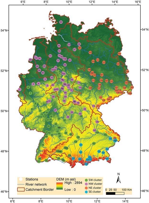
Water Resources Research 10.1029/2019WR025598

 Figure 1. Study area, main rivers including catchment boundaries, and location of the streamflow stations.

 the probability of flood occurrence starting from the atmospheric circulation features (Orton et al., 2018).
 We use streamflow data along the German hydrographic network, since Germany is well monitored with a
 sufficiently long record. Further, a number of studies have looked into the climate-flood link for this area,
 so our results can be compared to the existing knowledge. The article is organized as follows: in sections 2
 and 3 the data and study area are described, and in section 4 the methodology is presented. The results are
 discussed in section 5, and the conclusions and future developments are highlighted in section 6.

 2. Study Area
 The study area is Germany in Central Europe. It is bounded between the Alps to the south and the North
 Sea to the north and between the Oder River to the east and the valley of the Rhine to the west. Other large
 rivers are the Danube, the Elbe, and the Weser Rivers (Figure 1).
 Germany is characterized by a west-east gradient with increasing continental climate and a north-south
 gradients with increasing elevation. The superposition of both gradients leads to spatial patterns in tem-
 perature, snow cover, and rainfall with implications for streamflow and flood regimes. Moisture fluxes into
 the study area are dominated by westerly winds, and high intensity precipitation events are usually associ-
 ated with cyclonic weather patterns (Merz et al., 2018; Steirou et al., 2017). Approximately two thirds of the
 maximum annual floods across Germany occur in winter (Uhlemann et al., 2010). Catchments that show a
 distinct winter dominated flood regime are located in the west, from south to north, in the Rhine and the
 Weser basins (Merz et al., 2018). Catchments in the Elbe basin and some parts of the Danube basin show
 a more mixed regime with frequent winter floods but also substantial summer floods. During summer, the
 advection of warm and moist air masses from the Mediterranean, referred as Vb pattern (Zugstrasse Vb),
 occasionally leads to very intense precipitation events and severe flooding over south and east Germany.
 Catchments in the Danube basins in the Alpine and pre-Alpine region in the south of Germany show a clear
 summer flood regime with annual maxima caused by either snowmelt events or convective rainfall events.

CONTICELLO ET AL. 3 of 16

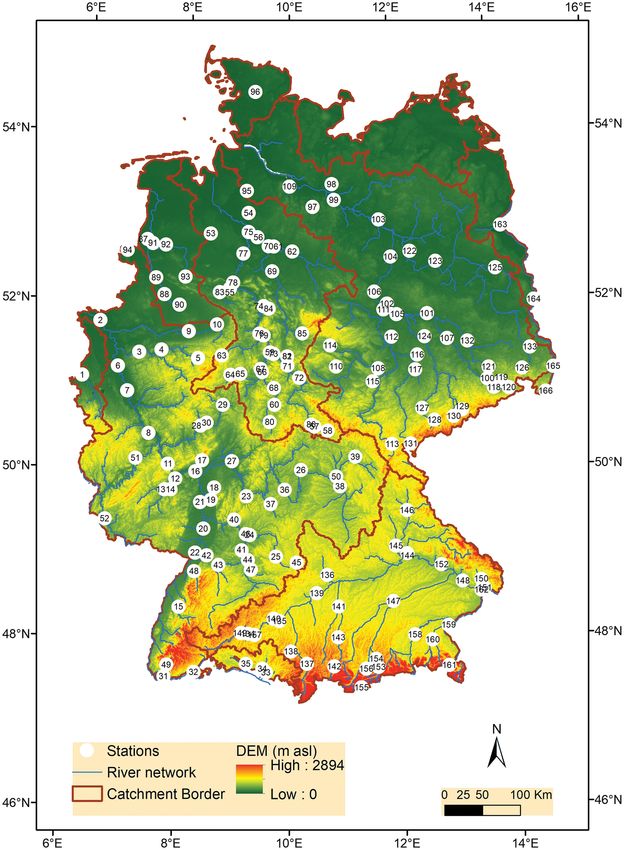
Water Resources Research 10.1029/2019WR025598

 Figure 2. Schematic of the methodology. (a) Data pretreatment to derive high streamflow events (HSE), integrated
 vapor transport (IVT), and circulation pattern (CP). (b) Sequence of the methods applied to derive clustered streamflow
 stations, HSE occurrence against CP, HSE occurrence against IVT, and HSE occurrence against both CP and IVT.

 3. Data
 The data used in this paper are the daily streamflow data, provided by the Global Runoff Data Center
 (GRDC), from 166 stations that cover homogeneously the whole of Germany (Figure 1). Data are available
 from 1 January 1960 to 31 December 2012. To represent atmospheric variables between 90◦ W and 70◦ E
 of longitude and 20◦ N and 80◦ N of latitude, we used daily data provided by the NCEP-NCAR Reanalysis
 (Kalnay et al., 1996): Geopotential height at 850 hPa, specific humidity, and zonal and meridional wind from
 1,000 to 300 hPa. The spatial resolution of the atmospheric fields is 2.5◦ for both latitude and longitude.

 4. Methods
 The methodology is shown in Figure 2. It consists of the following steps: (1) pretreatment of the stream-
 flow and atmospheric data to derive high streamflow events (HSEs), integrated vapor transport (IVT), and
 circulation patterns (CPs) (Figure 2a); (2) identification of HSE synchronized streamflow gauge clusters
 (Figure 2b); (3) evaluation of the link (synchronization) and time lag (delay) between HSEs and CPs for
 each cluster; (4) evaluation for each cluster of the relation between HSE and IVT value at the point of the
 reanalysis grid close to the geographic center of each cluster; and (5) assessment of the probability of HSE
 occurrence given CP and IVT for each cluster. Synchronization and delay between two binary variables (e.g.,
 gauge-gauge or gauge-CP) is evaluated by event synchronization (ES). Gauges and CPs with common behav-
 ior are pooled together using the modularity method; results are represented by complex networks. We use
 local regression to identify a relation between a binary variable (HSE) and a discrete variable (IVT). A Matlab
 code, available from the authors, was developed for calculating synchronization and delay between binary
 variables. Igraph R package (http://arxiv.org/abs/arXiv:0803.0476) is used to apply the modularity method.
 The Meteolab Meteorological toolbox for Matlab (https://meteo.unican.es/trac/MLToolbox/wiki) is used to
 apply SOM, whose output is a topologically ordered mapping of the input data, where similar patterns are

CONTICELLO ET AL. 4 of 16

Water Resources Research 10.1029/2019WR025598

Figure 3. Decomposition of the daily streamflow time series into seasonal, trend, and remainder components (left) and peak identification from the remainder
time series by selecting the discharge peak values exceeding the 90th percentile (right).

 mapped onto neighboring map regions, while dissimilar patterns are located further apart. Local regression
 relies on the R Package (http://r-statistics.co/Logistic-Regression-With-R.html). The methods are explained
 in more detail in the following sections.
 4.1. Definition of High Streamflow Events
 The method to derive high streamflow events (HSEs) relies on the peak identification method inspired by
 Uhlemann et al. (2010) which has been successfully applied to the Elbe River in Germany by Nied et al.
 (2014, 2017). We first decompose the discharge time series into seasonal, trend, and remainder components.
 We adopt the method proposed by Cleveland et al. (1990), known as Seasonal Decomposition of Time Series
 by Loess (STL). This procedure consists of a sequence of smoothing operations using loess, a locally weighted
 regression (Cleveland & Devlin, 1988). STL is used to identify the seasonality and long-term trend in a given
 time series. We retain the remainder component, on the base of the following motivations. The seasonal and
 trend components represent slow changes over time in the mean value of the streamflow. Consequently,
 the remainder represents anomalies relative to the seasonal mean and the long-term trend mean; that is,
 it is due to a perturbation of the mean and hence to an event above the baseline. HSEs are identified from
 the remainder time series by selecting the discharge peak values exceeding the 90th percentile. Figure 3
 exemplarily shows the results of the pretreatment and the peak detection. The left panel shows the recorded
 streamflow, the seasonal, trend, and remainder components. The right panel illustrates how the remainder
 is used to identify independent peaks (highlighted in red).
 First, two successive peaks are retained if they are separated by at least 3 days (Nied et al., 2014; Uhlemann
 et al., 2010). Then, in order to select only the peaks occurring during the buildup period in the hydrograph,
 which is the period in which the weather conditions influence the increase in the streamflow (Nied et al.,
 2014), we apply a moving average. Peaks are selected if they exceed a moving average with a time window
 of 15 days. This selection is applied to all stations shown in Figure 1. For each station, a binary time series is
 obtained, using 1 for peaks, 0 elsewhere. Hence, a binary matrix Ft,s (with t = 1, nT ; s = 1, nS ) is constructed
 where nT and nS are the number of time steps and streamflow gauges, respectively.
 4.2. Estimation of Integrated Vapor Transport
 Integrated vapor transport (IVT) is used to quantify the moisture transport in a region, that is, a cell of the
 reanalysis data set. It is estimated by integration over the air column, from 1,000 to 300 hPa, of the specific
 humidity multiplied by the zonal and meridional wind components:
 √
 300 300
 1 1
 IVT = qudp + qvdp
 g ∫1,000 g ∫1,000
 ,

CONTICELLO ET AL. 5 of 16

Water Resources Research 10.1029/2019WR025598

 where q is the specific humidity in kg∕kg, u is the zonal wind in m∕s, v is the meridional wind in m∕s, p is
 the pressure in hPa, and g is the acceleration due to gravity.

 4.3. Identification of Circulation Patterns
 Event synchronization applies to binary time series. Thus, geopotential height at 850 hPa (GPH850) anomaly
 time series have to be converted to a binary sequence to associate them with the streamflow peaks. This is
 done by (a) clustering the daily GPH850 anomaly fields into a number of representative circulation patterns
 (CPs); (b) assigning each day to the CP most similar to the GHP850 field of that day; and (c) constructing a
 binary matrix whose elements indicate the occurrence of a CP at a given day. The clustering of point (a) is
 carried out using Self Organized Map (SOM), that is, an unsupervised competitive learning neural network
 which projects the high-dimensional GPH850 data set onto a two-dimensional set of CPs. The Kaski and
 Lagus error criterion (Kaski & Lagus, 1996), which provides a global measure of both quantification and
 topological errors, is used to estimate the optimal number of CPs needed for an accurate representation of
 the daily GHP850 date set. A similar approach, based on the minimization of quantization and topographic
 errors, was also applied by Rousi et al. (2015). Applying the k-nearest neighbor method (Cover & Hart,
 1967), the daily GPH850 anomaly time series is substituted with the sequence of the CPs. Finally, a binary
 matrix Gt,g (t = 1, nT ; g = 1, nG ) is constructed in which the tth row indicates the day and the gth column
 the associate CP, being nT the number of time steps, and nG the number of CPs. The matrix element Gt,g is
 set equal to 1 if the specific configuration applies, 0 otherwise.

 4.4. Event Synchronization
 The two matrices Ft,s and Gt,g have the same number of rows, and they can be horizontally concatenated in
 a unique matrix Et,k , with t = nT , k = nE , and nE = nS + nG . Each column of the matrix Et,k is a time series of
 events, according to the definition given in the previous paragraphs. Given two binary time series of events,
 Ei,x and Ei,y , (where x and y indicate two different columns of Ei,k , x ≠ y), event synchronization quantifies
 the synchronization degree, that is, the number of near-simultaneous occurrence of events between the
 two time series, as well as the time delay of the events of a time series with respect to those of the other. A
 slightly different formulation from the one proposed by Quiroga et al. (2002) and Kreuz et al. (2015), given
 in Conticello et al. (2018), is used to compute the synchronization degree and the delay between each couple
 of time series of matrix Ei,k . Let xi (i = 1, 2, … , mx ) and yj (j = 1, 2, … , my ) be two vectors, each element of
 which identifies the time, tix and t , of occurrence of events in the respective time series; mx and my are the
 number of events in the vectors xi and yj , respectively. The two vectors xi and yj are obtainable from the time
 series Et,x and Et,y corresponding to two arbitrary chosen columns x and y of Et,k . Let s (x|y) and s (y|x) be the
 number of times an event appears in x shortly before or after it appears in y within a pre-fixed time window 
 m 
 ∑
 mx
 ∑
 s i (x| ) = Si ; s ( |x) = S (1)
 i=1 =1

 with Si = 1 if ∃ min(|tix − t ≤ |), and Si = 0 else. The conditional probability of an event x given the
 occurrence of an event y (and vice versa) can be calculated by

 s (x| ) s ( |x)
 P (x| = 1) = ; P ( |x = 1) = . (2)
 mx m 

 Furthermore, a measure of event synchronization is provided by

 s (x| ) + s ( |x)
 Q x, = . (3)
 mx + m 

 In order to explore the directionality of the delay, we define
 m 
 ∑
 mx
 ∑
 d (x| ) = Di ; d ( |x) = D (4)
 i=1 =1

 with Di = 1 if ∃ min(0 < tix − t ≤ ), and Di = 0 else. A measure of directionality of the delay can be
 expressed by

CONTICELLO ET AL. 6 of 16

Water Resources Research 10.1029/2019WR025598

 d (x| ) − d ( |x)
 q x, = . (5)
 mx + m 

 According to the definitions of equations (3) and (5), 0 ≤ Q x, ≤ 1 and −0.5 ≤ q x, ≤ 0.5. For Q x, = 1, events
 are fully synchronized, for q x, = −0.5, events in the y time series always anticipate events in x. Varying k
 from 1 to nE , the variables of equations (1) and (4) can be calculated to derive the synchronization and delay
 between pairs of streamflow gauges and between streamflow gauges and CPs. A nE x nE synchronization
 matrix Q x, and a nE x nE delay matrix Q x, , whose elements are calculated by equations (1) and (4), respec-
 tively, can be constructed. The matrices Q x, and Q x, describe the strength of the link between the elements
 and the directionality of the link, respectively.

 4.5. Complex Network Clustering by Modularity
 The nG CPs and nS streamflow gauges can be defined as nodes of a weighted and directed complex network
 (details are provided in supporting information), where the strength of connections between the nodes is
 given by the value of the elements of the synchronization matrix Q(i, j) . In order to explore if there is an
 underlying causal structure between CPs and HSEs, as well as between the HSEs at different streamflow
 gauges, we analyze the community structure of the complex networks; that is, we analyze if the nodes of
 the complex networks can be organized in clusters, where many links connect the nodes within a cluster,
 and comparatively few links exist between the nodes of different clusters. The modularity method (Blondel
 et al., 2008; Newman, 2004) is applied to identify communities into which a complex network can be split.
 Modularity is based on the comparison between the actual density of links inside a community and the
 density one would expect if the nodes were attached at random, regardless of the community structure.
 Modularity M is calculated by
 [ ∏∏ ]
 1 ∑ i 
 M= Qi, − (ci , c ), (6)
 2m i, 2m

 ∏ ∑
 where Qij represents the strength of the link between the nodes i and j, i = Qi is the sum of the strength
 of the links attached to node i, ci is the community to which node i is assigned, the − function (u, v) is
 ∑
 1 if u = v and 0 otherwise, and m = 12 i Qi . Equation (6) is solved using the two-step iterative algorithm
 proposed by Blondel et al. (2008), also known as Louvain Method. In the present study, the modularity
 method is applied twice. First, it is applied to the HSEs associated to the entire set of streamflow gauges. In
 this way a number of communities of streamflow gauges with strong HSE synchronization are identified.
 Then the modularity method is applied again, separately for each community, to assess the link between
 HSEs and CPs.

 4.6. HSE-IVT Local Regression
 Local regression (Loader, 1999), based on generalized linear models (glm) with Bernoulli response and link
 logit, is used to compute the probability of HSE occurrence given IVT as predictor. The problem can be
 formulated as follows. Let Y = (y1 , … , yn ) be a binary time series, defined by
 {
 1 if there is at least one HSE in the group of streamflow considered,
 i = (7)
 0 otherwise,

 where i is the value of y at the ith time step. Let xi = (xi1 , … , xip ) be the predictor time series, whose elements
 are the IVT values, at the ith time step, of the cell of the NCEP-NCAR Reanalysis data closest to the centroid
 of the streamflow gauge community. Being i = E(Yi |xi ), a glm can be specified for Y

 g( i ) = 0 + 1 xi1 + … + p xip = i , (8)

 where i is the linear predictor and g(·) is the link function. A Bernoulli distribution is used to identify the
 binary response variable:

 P(Yi = 1) = i P(Yi = 0) = 1 − i . (9)

CONTICELLO ET AL. 7 of 16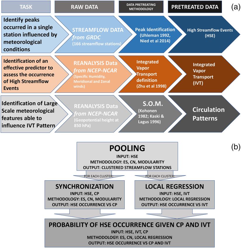

Water Resources Research 10.1029/2019WR025598

 Figure 4. Clusters of streamflow stations based on event synchronization and modularity. Clusters are represented by
 different colors.

 Since i is defined between 0 and 1, a logistic transform can be used as a link function:
 ( )
 i
 g( i ) = ln = 0 + 1 xi1 + … + p xip = i . (10)
 1 − i

 To estimate i , the link function is inverted:
 e i
 i = . (11)
 1 − e i

 Further details on HSE-IVT local regression are provided in the supporting information.

 5. Results and Discussion
 5.1. Pooling Streamflow Stations in Homogeneous Clusters
 Figure 4 shows the main rivers, their basin boundaries, and the complex network of the streamflow stations
 based on event synchronization and modularity. The nodes represent the stations, and the links indicate
 synchronization between HSEs. Four clusters of stations are identified. To a large part, as expected, these
 clusters coincide with the main German river basins: South Western Rhine (green), North Western/Central
 Weser (pink), North Eastern Elbe (orange), and South Eastern Danube (blue). The few exceptions are related
 to streamflow stations assigned to an adjacent basin, where the membership is caused by the spatial distribu-
 tion of rainfall events due to the storm orientation generating floods that do not overlap with the boundaries
 of the basins.
 5.2. Local Regression to Relate High Streamflow Events and Integrated Vapor Transport
 After the pooling, we study the influence of integrated vapor transport (IVT) on the probability of occurrence
 of a heavy streamflow event (HSE) by applying local logistic regression to the binary sequence of HSEs and
 the corresponding IVT. In Figure 5 the results of this analysis are presented for the four clusters.

CONTICELLO ET AL. 8 of 16

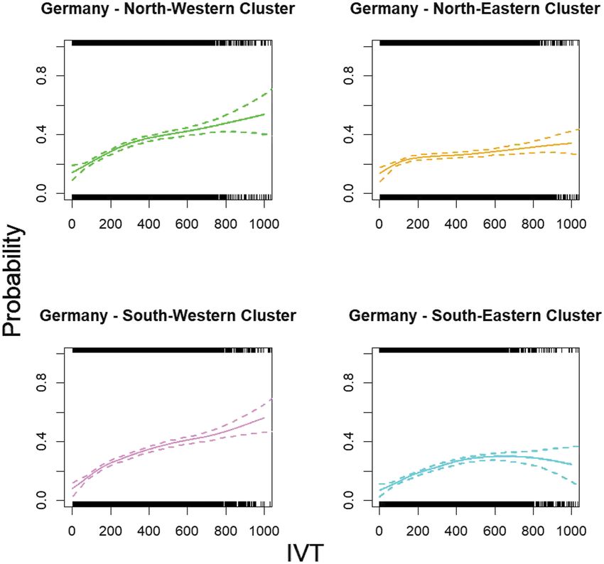
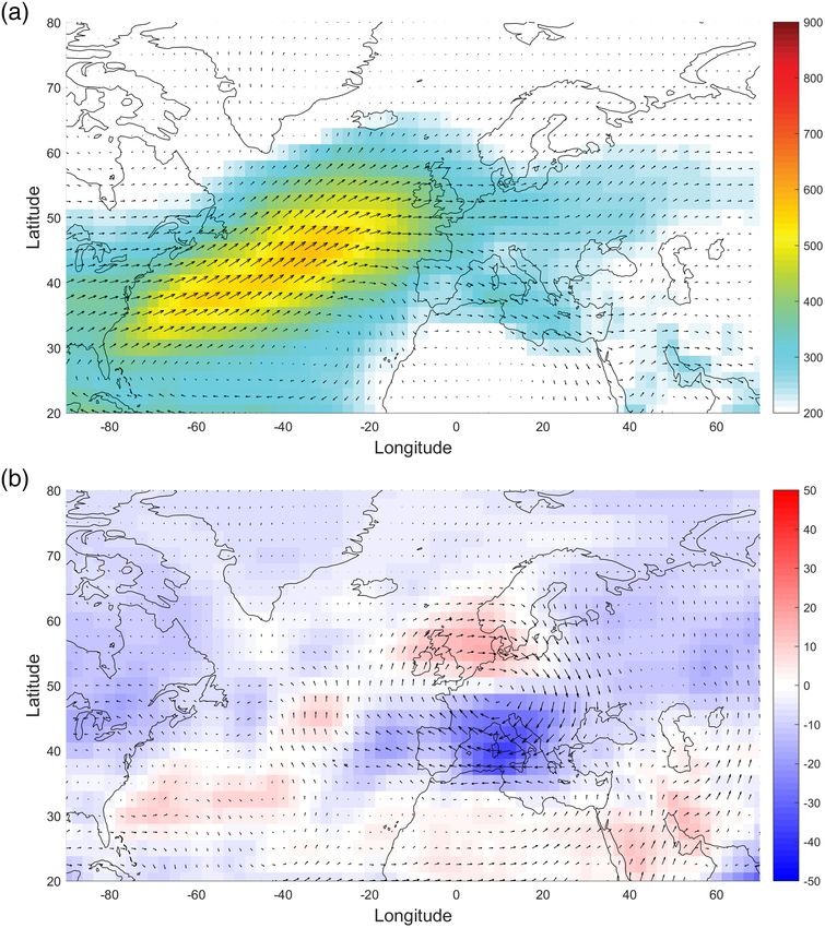
Water Resources Research 10.1029/2019WR025598

 Figure 5. Probability of occurrence of at least one high streamflow event (HSE) within the four station clusters as
 function of integrated vapor transport (IVT). IVT values are obtained taking the closest cell value to the centroid of
 each cluster. Dashed lines: 95% confidence band. At the top and the bottom of each figure, HSE occurrence is
 represented with 0 (bottom: it means that HSE didn't overpass the threshold) and 1 (top: it means that HSE overpassed
 the threshold) associated to IVT values.

 All clusters show a dependence of the probability of HSE occurrence on IVT which suggests that IVT is a
 useful predictor for river flooding. This agrees with the literature on the influence of moisture transport on
 the probability of extreme precipitation or flooding and in particular on the effectiveness of IVT as an early
 warning indicator (Lavers et al., 2012; Lavers & Villarini, 2013). However, for high IVT values the probability
 of having at least one high streamflow event in the region is higher for the western regions than in eastern
 regions. Figure 6a shows the composite of wind and IVT for the HSEs in the northwestern cluster, while
 Figure 6b shows the difference between the composites of the northwestern and southwestern clusters. For
 both regions, HSE occurrences are related to similar wind and IVT patterns. However, small shifts in these
 patterns at the synoptic scale, highlighted in Figure 6b, can result in a deflection of moisture transport that
 is sufficient to cause heavy rainfall (at the spatial scale of Germany) in another region.
 Figure 6 shows that HSE occurrence in these regions is mainly related to westerly moisture flux. This
 observation is consistent with the widespread understanding that flooding in Central Europe is primarily
 associated with geopotential states that favor westerly moisture flows (e.g., Blöschl et al., 2017; Bendix, 2017;
 Jacobeit et al., 2003; Steirou et al., 2017, 2019). In supporting information are reported Figures S1–S3, simi-
 lar to Figure 6, but showing the difference of IVT and wind between eastern and north-western clusters. The
 mechanism of moisture transport able to generate high streamflow in the southern eastern cluster differs
 significantly from the one affecting the other clusters. Indeed, in this region the moisture transport is often
 linked to so-called Vb cyclones that usually occur in late Spring and Summer, bringing warm and humid air
 masses advected from south Europe northward to Central and Eastern Europe (Jacobeit et al., 2006; Nied
 et al., 2014; Petrow et al., 2007; Ulbrich et al., 2003).

 5.3. Self Organizing Maps to Identify Circulation Patterns
 To identify the atmospheric pressure patterns that influence the transport of moisture during HSEs, we ana-
 lyze the daily geopotential fields at 850 hPa. We reduce the data set of over 20,000 daily geopotential height

CONTICELLO ET AL. 9 of 16

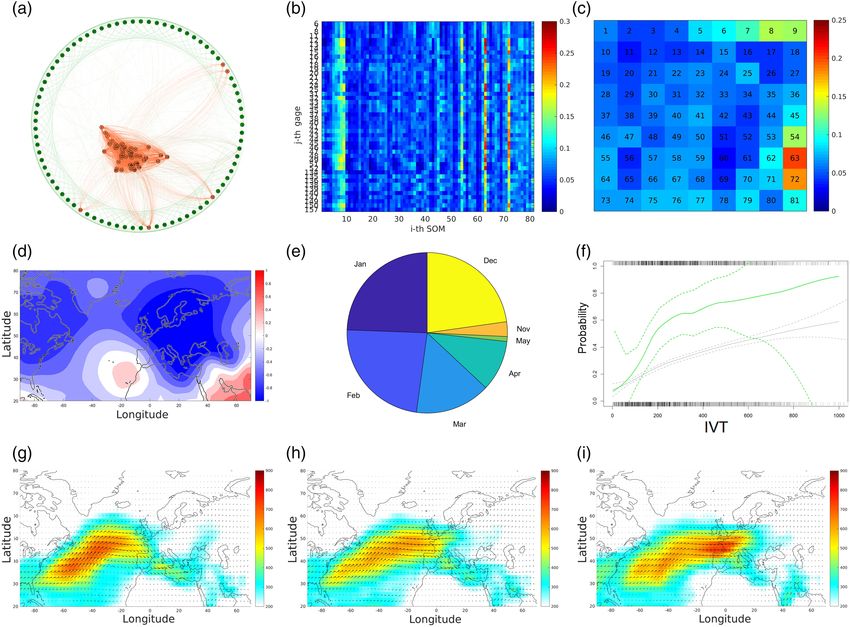
Water Resources Research 10.1029/2019WR025598

 Figure 6. IVT composite for high streamflow events occurring in the north-western/central cluster (a). Difference
 between IVT composites of the northwestern and southwestern clusters (b). Arrows show the wind direction and
 speed, colors code IVT. It is evident that westerly moisture flow influences high streamflow events in both clusters.

 fields using Self Organizing Maps (SOMs). The error function (Kaski & Lagus, 1996) is given in Figure S4
 in supporting information, showing the error versus the number of maps necessary to synthesize the origi-
 nal data set. Figure 7 shows the resulting 81 circulation patterns for the optimal tradeoff between number
 of maps and error. The resulting number of 81 CPs is rather high compared to other circulation type clas-
 sifications. There are some similarities between different CPs, but a subtle shift in circulation patterns may
 translate into streamflow impact in a different watershed (see also section 5.2). The small shifts that are seen
 between similar CPs correspond physically to the wave guide centered in the case of the CPs that matter
 most for HSE on Germany.

 5.4. Synchronization and Local Regression to Relate High Streamflow Events With Circulation
 Patterns and Integrated Vapor Transport
 The relations between HSEs and CPs and IVT are studied for each cluster. The results for the south-western
 cluster are shown in Figure 8.
 Figure 8a shows a complex network whose nodes at the center of the circle represent the streamflow stations
 of the south-western cluster, while the nodes arranged in the outer circle represent the 81 circulation pat-
 terns. The presence, or absence, of links between the nodes indicates their synchronization Q. Circulation
 patterns 8, 9, 54, 63, and 72 are highly synchronized with the HSEs of this cluster. To identify the circulation
 pattern which shows the strongest synchronization, we plot the values of the synchronization between each

CONTICELLO ET AL. 10 of 16

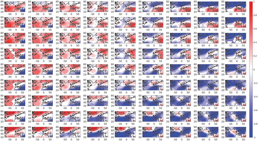
Water Resources Research 10.1029/2019WR025598

Figure 7. Self Organizing Maps (SOM) for the geopotential height at 850 hPa.

 station and each circulation pattern (Figure 8b). Circulation patterns 63 and 72 stand out as highly synchro-
 nized. Averaging across all stations of the south-western cluster shows that circulation pattern 63 is the most
 synchronized pattern with HSEs (Figure 8c). This pattern, consisting of a GPH850-positive anomaly around
 the Canary Islands and negative ones on Central Europe with the strongest gradient around the Pyrenees,
 generates winds whose average speeds are highest at the latitudes where Germany is located (Figure 8d).
 This circulation pattern occurs about five to six times per year. In almost 75%, it occurs in winter (DJF). If we
 also include March and April, we reach >90% (Figure 8e). The local logistic regression function, which links
 the probability of HSE occurrence to IVT, for configuration 63 shows an increase in the regression slope in
 the IVT interval from 0 to 250 kg m−1 s−1 compared to all circulation patterns (Figure 8f). This translates
 into much higher probability values for IVT larger than around 100 kg m−1 s−1 For example, the probabil-
 ity of occurrence of a HSE in the south-western cluster for an IVT value of 300 kg m−1 s−1 is 30%, while
 it reaches over 60% if conditioned on CP 63. It is evident that knowing both the value of moisture trans-
 port and the geopotential configuration leads to a significant improvement in the predictive capacity of the
 model. As expected, due to the minor number of data of the time series, the confidence intervals for the CP
 conditioned local logistic regression (Figure 8f) are wider than non CP conditioned ones. However, the con-
 fidence intervals significantly diverge only for very extreme value of IVT, which don't question the previously
 discussed finding. Figures 8g–8i show the IVT composites obtained by sampling the IVT fields during the
 circulation pattern 63 for different ranges of IVT values. These figures illustrate the reason why taking both
 variables into account improves the model skill. While IVT gives an idea of the local moisture concentration,
 the geopotential state provides information on the path followed by the humidity, especially from where it
 originates and where it moves to. The results for the north-western/central cluster (Figure S5 in supporting
 information) are very similar to those for the south-western cluster. These clusters mostly coincide with the
 Rhine and Weser basins, which have a distinct winter flood regime (Belz et al., 2007; Beurton & Thieken,
 2009; Disse & Engel, 2001; Mudelsee et al., 2004; Petrow et al., 2009). For the north-eastern cluster (Figure
 S6 in supporting information), which coincides with the Elbe basin, the results (supporting information)
 are similar to those of the two western clusters, although the synchronization between HSEs and circula-
 tion patterns is lower. The most important circulation pattern for this area is 72. Compared to 63, the pattern

CONTICELLO ET AL. 11 of 16

Water Resources Research 10.1029/2019WR025598

Figure 8. (a) Complex networks for the south-western cluster. Nodes at the center represent streamflow stations of the south-western cluster, while the nodes
at the outer circle represent the 81 circulation patterns. (b) Synchronization matrix between high streamflow events of this cluster and CPs. (c) Mean
synchronization matrix, averaged across all streamflow stations. (d) Most synchronized circulation pattern: CP 63. (e) Seasonal distribution of the occurrence of
CP 63. (f) Local logistic regression for CP 63: probability of occurrence of at least one HSE in the south-western cluster as function of IVT. (g–i) IVT composites
during CP 63 for different values of IVT: 100–300 (g), 300–500 (h), >500 (i).

 72 has the center of the higher positive geopotential values moved to the north, 20◦ W, 45◦ N. This pattern
 collects moisture from the north Atlantic not immediately discharging it to the west of the French coast, as
 it happens with the pattern 63, but deviating to the north and arriving directly in the north-eastern cluster.
 This result agrees with Uhlemann et al. (2010) and Petrow et al. (2007) who also found that this region is
 affected during winter floods by similar circulation patterns, albeit less, to those that activate floods in the
 west of the country. The south-eastern cluster (Figure S7 in supporting information), on the other hand, has
 the HSE synchronized with the circulation patterns ordered along the left column of the map matrix, corre-
 sponding to summer patterns. Conditioning the HSE occurrence versus IVT regression to a specific CP does
 not increase the probability of HSE occurrence. The IVT composites for values greater than 500 kg m−1 s−1
 show the presence of moisture in Central Europe without indicating a preferential route of transport from
 other regions. This result can be explained by the variety of flood generation processes in that portion of the
 Danube basin. Floods typically occur in summer, often caused by convective rainfall events (Prudhomme
 & Genevier, 2011), but snowmelt and large-scale frontal systems play an important role as well. Merz et al.
 (2018) note that extreme summer floods in this region are often associated with Vb storm tracks which favor
 moisture transport from the Mediterranean and in particular from the Gulf of Genoa and the Adriatic sea.
 The synoptic situation of a Vb system is, by and large, characterized by high pressure centers on the English
 Channel and lows on the Gulf of Genoa and Alps. The persistence of this situation increases the residence

CONTICELLO ET AL. 12 of 16

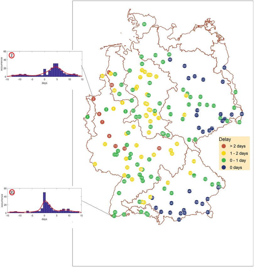
Water Resources Research 10.1029/2019WR025598

 Figure 9. Delay values, q, for each station associated with CP 63, that is, the circulation pattern which is most
 synchronized with HSEs in Germany. Colors indicate the delay value for each station, from low (blue) to high (red).
 Histograms of delay values are shown for two stations. Station 31 in the mountainous part of the Rhine basin has most
 often a delay of zero; that is, HSEs occur on the same day as CP 63. At station 2, the most downstream gauge of the
 Rhine River, the most frequent delay is between 4 and 5 days.

 time of a Vb cyclone and thus the amount of precipitation over Central Europe. In addition, Merz et al. (2018)
 found that the initial catchment state plays a much larger role for flood generation in this region compared
 to other river basins in Germany. Similarly, Blöschl et al. (2013) observed that the particularly disastrous
 summer floods of 1954, 2002, and 2013 for the Danube started after extended rainy periods which saturated
 the ground. Since our indicators CP and IVT do not represent the initial catchment conditions, our model is
 less well suited for this cluster. Here, an approach similar to Nied et al. (2014) who attempt to consider the
 atmospheric situation jointly with the initial catchment state should be developed.

 5.5. Synchronization and Delay to Identify Optimal Time Window
 In addition to synchronization values, event synchronization also provides delay values (equation (5)).
 Figure 9 shows the map of delay values between streamflow peaks and the most synchronized circulation
 pattern with the western clusters (CP 63).
 As expected, the delay values increase along the hydrograph network of each basin from upstream to down-
 stream regions. We select two stations of the south-western cluster, namely, stations 31 and 2 indicated with
 a red circle in the delay map to demonstrate the capability of the method to detect complex spatiotemporal
 relations. For these stations, histograms of the frequency versus lag time between the occurrence of CP 63
 and of HSE, within the time window, were calculated. Station 31 is located in the mountainous areas of the
 Rhine. Its histogram has its highest value for a delay equal to 0; that is, the HSEs occur on the same day as
 the CP 63. The histogram of station 2 which is the most downstream station at the Rhine, instead, shows
 a peak corresponding to delay values of 4 to 5 days. This is coherent with the physics of the system which
 suggests that downstream gauges have longer delay than upstream gauges.

CONTICELLO ET AL. 13 of 16

Water Resources Research 10.1029/2019WR025598

 6. Conclusions
 The goal of this research was to identify, considering an appropriate delay, the atmospheric circulation fea-
 tures and moisture transport patterns that cause space-time peaks in streamflow, and to use this information
 for linking the probabilistic occurrence of high streamflow events to these large-scale climate features. To
 this end, we extended the methodology recently proposed by Conticello et al. (2018) for assessing the proba-
 bility of heavy rainfall occurrence. Using river discharge records from streamflow gauges covering the entire
 German territory, we showed that the proposed methodology can be successfully applied to (a) identify the
 atmospheric patterns most synchronized to HSE occurrence; (b) find a significant statistical dependence,
 by logistic regression, between the probability of occurrence of HSE and the IVT in the examined regions,
 conditioned on the CPs most synchronized with HSEs of the streamflow clusters; (c) use event synchroniza-
 tion not only to identify the CPs most synchronized to HSEs but also through the delay values to identify a
 clear causality between CP and HSE occurrence; and (d) calculate the delay between CP and HSE which is
 embedded in the calculation and could subsequently be used in the prediction. Some relevant aspects of the
 proposed methodology can be highlighted:
 • We found a statistically significant dependence of HSE occurrence on the local values of IVT, conditional
 to the most synchronized CP. This approach improves a probabilistic approach that links HSE occurrence
 only to the local IVT as proposed by Lavers and Villarini (2013).
 • Very high probabilities of HSE occurrence (conditioned on the most synchronized CP), as a function of
 local value of IVT, were found for most of the clusters identified by event synchronization and modu-
 larity. This is particularly evident for the two western clusters where floods are driven by atmospheric
 circulation patterns represented by a positive anomaly around the Canary Islands and negative ones at
 Central Europe with strongest gradient around the Pyrenees. Such fields are associated to winds whose
 average speeds are highest at the latitudes where western Germany is located and that are able to transport
 moisture along atmospheric rivers, originating in the Tropics.
 • The dependence of HSE occurrence on the proposed atmospheric predictors suggests the possibility to
 construct flood early warning tools or to assess changes in HSE frequency due to the occurrence of more
 frequent atmospheric circulation patterns able to generate floods or due to an increase of humidity in the
 atmospheric column as expected in the future.
 Some limitations of the approach are noted. Our analysis is limited to high streamflow events that are linked
 to rainfall involving large-scale atmospheric circulation. For the south-eastern cluster, only a weak depen-
 dence of HSE occurrence on IVT could be found. This is explained by the flood generation processes in
 these regions. Floods typically occur in summer often caused by local convective rainfall events or snowmelt
 and where the soil saturation may play a larger role in generating HSEs. To overcome such limitation, an
 upgrade of the approach is necessary further investigation need. Large-scale circulation is represented by
 nodes obtained by SOM. The number of patterns represents a tradeoff between bias and variance in identify-
 ing groups. While a large number of CPs were retained, only a few CPs are highly synchronized with HSEs,
 and these are statistically significant predictors in the logistic regression. Our analysis is limited to a sym-
 metric SOM and to a given spatial domain. We identify the number of nodes on the basis of the variance of
 only geopotential time series and not by including the link with HSE. This has the advantage that the CPs
 are identified independently of the HSEs and then a small subset that influences the extreme HSEs can be
Acknowledgments identified. This approach mitigates the overfitting that could result if the HSEs were used to train the clus-
We would like to acknowledge Dr. tering of the CPs. However, there is room for refining the proposed methodology exploring non-symmetrical
Nguyen Viet Dung for his precious
 SOM and spatial domain of different extension. A relevant result of our study is the identification of the two
work to provide Figures 1 and 9.
Streamflow Data were provided by The significant atmospheric predictors IVT and GPH850. Classifying GPH and IVT patterns together to explore
Global Runoff Data Centre, 56068 the existence of a stronger link with HSE could be a further possibility, as well as the choice of a smaller
Koblenz, Germany, and it is available
 region to apply the methodology.
online (at https://www.bafg.de/GRDC/
EN/02&urluscore;srvcs/21&urluscore;
tmsrs/riverdischarge&urluscore;node.
html) (accessed 30/01/2020). NCEP
 References
NCAR Reanalysis data are available at Allan, R. P., Lavers, D. A., & Champion, A. J. (2016). Diagnosing links between atmospheric moisture and extreme daily precipitation over
the IRI Climate Data Library (https:// the UK. International Journal of Climatology, 36(9), 3191–3206.
iridl.ldeo.columbia.edu/SOURCES/. Allan, R. P., Liu, C., Zahn, M., Lavers, D. A., Koukouvagias, E., & Bodas-Salcedo, A. (2014). Physically consistent responses of the global
NOAA/.NCEP-NCAR/.CDAS-1/. atmospheric hydrological cycle in models and observations. Surveys in Geophysics, 35(3), 533–552.
DAILY/) (accessed 30/01/2020). The Bárdossy, A. (2010). Atmospheric circulation pattern classification for South-West Germany using hydrological variables. Physics and
authors declare that they have no Chemistry of the Earth, Parts A/B/C, 35(9-12), 498–506.
conflict of interest. Barredo, J. I. (2007). Major flood disasters in Europe: 1950–2005. Natural Hazards, 42(1), 125–148.

CONTICELLO ET AL. 14 of 16

Water Resources Research 10.1029/2019WR025598

 Belz, J. U., Brahmer, G., Buiteveld, H., Engel, H., Grabher, R., Hodel, H., et al. (2007). Das Abflussregime des Rheins und seiner Nebenflüsse
 im 20. Jahrhundert: Analyse, Veränderungen, Trends. Internationale Kommission für die Hydrologie des Rheingebietes.
 Bendix, J. (1997). Natürliche und anthropogene Einflüsse auf den Hochwasserabfluss des Rheins natural and human impacts on flood
 discharge of the river Rhine. Erdkunde, Bd. 51(H. 4), 292–308.
 Beurton, S., & Thieken, A. H. (2009). Seasonality of floods in Germany. Hydrological Sciences Journal, 54(1), 62–76.
 Bhalme, H. N., & Mooley, D. A. (1980). Large-scale droughts/floods and monsoon circulation. Monthly Weather Review, 108(8), 1197–1211.
 Blöschl, G., Hall, J., Parajka, J., Perdigão, R. A., Merz, B., Arheimer, B., et al. (2017). Changing climate shifts timing of European floods.
 Science, 357(6351), 588–590.
 Blöschl, G., Nester, T., Komma, J., Parajka, J., & Perdigão, R. (2013). The June 2013 flood in the Upper Danube basin, and comparisons
 with the 2002, 1954 and 1899 floods. Hydrology and Earth System Sciences, 17(12), 5197–5212.
 Blondel, V. D., Guillaume, J.-L., Lambiotte, R., & Lefebvre, E. (2008). Fast unfolding of communities in large networks. Journal of Statistical
 Mechanics: Theory and Experiment, 2008(10), P10008.
 Cleveland, R. B., Cleveland, W. S., McRae, J. E., & Terpenning, I. (1990). STL: A seasonal-trend decomposition. Journal of Official Statistics,
 6(1), 3–73.
 Cleveland, W. S., & Devlin, S. J. (1988). Locally weighted regression: An approach to regression analysis by local fitting. Journal of the
 American Statistical Association, 83(403), 596–610.
 Conticello, F., Cioffi, F., Merz, B., & Lall, U. (2018). An event synchronization method to link heavy rainfall events and large-scale
 atmospheric circulation features. International Journal of Climatology, 38(3), 1421–1437.
 Cover, T. M., & Hart, P. E. (1967). Nearest neighbor pattern classification. IEEE Transactions on Information Theory, 13(1), 21–27.
 Dacre, H. F., Clark, P. A., Martinez-Alvarado, O., Stringer, M. A., & Lavers, D. A. (2015). How do atmospheric rivers form? Bulletin of the
 American Meteorological Society, 96(8), 1243–1255.
 Desai, B., Maskrey, A., Peduzzi, P., De Bono, A., & Herold, C. (2015). Making development sustainable: The future of disaster risk
 management, global assessment report on disaster risk reduction.
 Disse, M., & Engel, H. (2001). Flood events in the Rhine basin: Genesis, influences and mitigation. Natural Hazards, 23(2-3), 271–290.
 Garaboa-Paz, D., Eiras-Barca, J., Huhn, F., & Pérez-Muñuzuri, V. (2015). Lagrangian coherent structures along atmospheric rivers. Chaos:
 An Interdisciplinary Journal of Nonlinear Science, 25(6), 063,105.
 Gerstengarbe, F.-W., & Werner, P. C. (2005). Simulationsergebnisse des regionalen klimamodells star. Auswirkungen des globalen Wandels
 auf Wasser, Umwelt und Gesellschaft im Elbegebiet. Konzepte für die nachhaltige Entwicklung einer Flusslandschaft, 6, 110–118.
 Hess, P., & Brezowsky, H. (1977). Katalog der Großwetterlagen Europas 1881-1976. 3. verbesserte und ergänzte Aufl. Berichte des Deutschen
 Wetterdienstes, 113, 1–140.
 Huth, R., Beck, C., Philipp, A., Demuzere, M., Ustrnul, Z., Cahynová, M., et al. (2008). Classifications of atmospheric circulation patterns.
 Annals of the New York Academy of Sciences, 1146(1), 105–152.
 Ionita, M., Lohmann, G., & Rimbu, N. (2008). Prediction of spring Elbe discharge based on stable teleconnections with winter global
 temperature and precipitation. Journal of Climate, 21(23), 6215–6226.
 Jacobeit, J., Glaser, R., Luterbacher, J., & Wanner, H. (2003). Links between flood events in Central Europe since AD 1500 and large-scale
 atmospheric circulation modes. Geophysical Research Letters, 30(4), 1172.
 Jacobeit, J., Philipp, A., & Nonnenmacher, M. (2006). Atmospheric circulation dynamics linked with prominent discharge events in Central
 Europe. Hydrological Sciences Journal, 51(5), 946–965.
 Jain, S., & Lall, U. (2000). Magnitude and timing of annual maximum floods: Trends and large-scale climatic associations for the Blacksmith
 Fork River, Utah. Water Resources Research, 36(12), 3641–3651.
 Kalnay, E., Kanamitsu, M., Kistler, R., Collins, W., Deaven, D., Gandin, L., et al. (1996). The NCEP/NCAR 40-year reanalysis project.
 Bulletin of the American Meteorological Society, 77(3), 437–472.
 Karamperidou, C., Cioffi, F., & Lall, U. (2012). Surface temperature gradients as diagnostic indicators of midlatitude circulation dynamics.
 Journal of Climate, 25(12), 4154–4171.
 Kaski, S., & Lagus, K. (1996). Comparing self-organizing maps. In International conference on artificial neural networks, Springer,
 pp. 809–814.
 Kreuz, T., Mulansky, M., & Bozanic, N. (2015). SPIKY: A graphical user interface for monitoring spike train synchrony. Journal of
 Neurophysiology, 113(9), 3432–3445.
 Lamb, H. H. (1972). British Isles weather types and a register of the daily sequence of circulation patterns 1861-1971. Her Majesty's
 stationery office.
 Lavers, D. A., & Villarini, G. (2013). The nexus between atmospheric rivers and extreme precipitation across Europe. Geophysical Research
 Letters, 40, 3259–3264. https://doi.org/10.1002/grl.50636
 Lavers, D. A., & Villarini, G. (2015). The contribution of atmospheric rivers to precipitation in Europe and the United States. Journal of
 Hydrology, 522, 382–390.
 Lavers, D. A., Villarini, G., Allan, R. P., Wood, E. F., & Wade, A. J. (2012). The detection of atmospheric rivers in atmospheric reanalyses
 and their links to British winter floods and the large-scale climatic circulation. Journal of Geophysical Research, 117, D20106. https://
 doi.org/10.1029/2012JD018027
 Lavers, D. A., Waliser, D. E., Ralph, F. M., & Dettinger, M. D. (2016). Predictability of horizontal water vapor transport relative to precipita-
 tion: Enhancing situational awareness for forecasting western US extreme precipitation and flooding. Geophysical Research Letters, 43,
 2275–2282. https://doi.org/10.1002/2016GL067765
 Lehner, B., Döll, P., Alcamo, J., Henrichs, T., & Kaspar, F. (2006). Estimating the impact of global change on flood and drought risks in
 Europe: A continental, integrated analysis. Climatic Change, 75(3), 273–299.
 Loader, C. (1999). Local regression and likelihood. New York, Berlin, and Heidelberg: Springer.
 Merz, B., Aerts, J., Arnbjerg-Nielsen, K., Baldi, M., Becker, A., Bichet, A., et al. (2014). Floods and climate: Emerging perspectives for flood
 risk assessment and management. Natural Hazards and Earth System Sciences, 14(7), 1921–1942.
 Merz, R., & Blöschl, G. (2003). A process typology of regional floods. Water Resources Research, 39(12), 1340.
 Merz, B., Dung, N. V., Apel, H., Gerlitz, L., Schröter, K., Steirou, E., & Vorogushyn, S. (2018). Spatial coherence of flood-rich and flood-poor
 periods across Germany. Journal of Hydrology, 559, 813–826.
 Merz, B., Kundzewicz, Z. W., Delgado, J., Hundecha, Y., & Kreibich, H. (2018). Detection and attribution of changes in flood hazard and
 risk, Changes in flood risk in europe (pp. 445–468). London: CRC Press.
 Mudelsee, M., Börngen, M., Tetzlaff, G., & Grünewald, U. (2004). Extreme floods in Central Europe over the past 500 years: Role of cyclone
 pathway “Zugstrasse Vb”. Journal of Geophysical Research, 109, D23101. https://doi.org/10.1029/2004JD005034

CONTICELLO ET AL. 15 of 16

Water Resources Research 10.1029/2019WR025598

 Murawski, A., Bürger, G., Vorogushyn, S., & Merz, B. (2016). Can local climate variability be explained by weather patterns?A multi-station
 evaluation for the Rhine basin. Hydrology and Earth System Sciences, 20(10), 4283–4306.
 Newell, R. E., Newell, N. E., Zhu, Y., & Scott, C. (1992). Tropospheric rivers?—A pilot study. Geophysical Research Letters, 19(24), 2401–2404.
 Newman, M. E. (2004). Analysis of weighted networks. Physical Review E, 70(5), 056,131.
 Nied, M., Pardowitz, T., Nissen, K., Ulbrich, U., Hundecha, Y., & Merz, B. (2014). On the relationship between hydro-meteorological
 patterns and flood types. Journal of Hydrology, 519, 3249–3262.
 Nied, M., Schröter, K., Lüdtke, S., Nguyen, V. D., & Merz, B. (2017). What are the hydro-meteorological controls on flood characteristics?
 Journal of Hydrology, 545, 310–326.
 Orton, P. M., Conticello, F. R., Cioffi, F., Hall, T. M., Georgas, N., Lall, U., et al. (2018). Flood hazard assessment from storm tides, rain and
 sea level rise for a tidal river estuary. Natural Hazards. https://doi.org/10.1007/s11069-018-3251-x
 Petrow, T., Merz, B., Lindenschmidt, K.-E., & Thieken, A. (2007). Aspects of seasonality and flood generating circulation patterns in a
 mountainous catchment in south-eastern Germany. Hydrology and Earth System Sciences Discussions, 4(2), 589–625.
 Petrow, T., Zimmer, J., & Merz, B. (2009). Changes in the flood hazard in Germany through changing frequency and persistence of
 circulation patterns. Natural Hazards and Earth System Sciences, 9(4), 1409–1423.
 Philipp, A., Bartholy, J., Beck, C., Erpicum, M., Esteban, P., Fettweis, X., et al. (2010). Cost733cat—A database of weather and circulation
 type classifications. Physics and Chemistry of the Earth, Parts A/B/C, 35(9-12), 360–373.
 Prudhomme, C., & Genevier, M. (2011). Can atmospheric circulation be linked to flooding in Europe? Hydrological Processes, 25(7),
 1180–1190.
 Quiroga, R. Q., Kreuz, T., & Grassberger, P. (2002). Event synchronization: A simple and fast method to measure synchronicity and time
 delay patterns. Physical Review E, 66(4), 041,904.
 Rousi, E., Anagnostopoulou, C., Tolika, K., & Maheras, P. (2015). Representing teleconnection patterns over Europe: A comparison of SOM
 and PCA methods. Atmospheric research, 152, 123–137.
 Rutz, J. J., Steenburgh, W. J., & Ralph, F. M. (2014). Climatological characteristics of atmospheric rivers and their inland penetration over
 the western United States. Monthly Weather Review, 142(2), 905–921.
 Steinschneider, S., & Lall, U. (2015a). Daily precipitation and tropical moisture exports across the eastern United States: An application of
 archetypal analysis to identify spatiotemporal structure. Journal of Climate, 28(21), 8585–8602.
 Steinschneider, S., & Lall, U. (2015b). A hierarchical Bayesian regional model for nonstationary precipitation extremes in Northern
 California conditioned on tropical moisture exports. Water Resources Research, 51, 1472–1492. https://doi.org/10.1002/2014WR016664
 Steirou, E., Gerlitz, L., Apel, H., & Merz, B. (2017). Links between large-scale circulation patterns and streamflow in Central Europe: A
 review. Journal of Hydrology, 549, 484–500.
 Steirou, E., Gerlitz, L., Apel, H., Sun, X., & Merz, B. (2019). Climate influences on flood probabilities across Europe. Hydrology and Earth
 System Sciences, 23(3), 1305–1322.
 Trenberth, K. E., & Guillemot, C. J. (1996). Physical processes involved in the 1988 drought and 1993 floods in North America. Journal of
 Climate, 9(6), 1288–1298.
 Uhlemann, S., Thieken, A., & Merz, B. (2010). A consistent set of trans-basin floods in Germany between 1952–2002. Hydrology and Earth
 System Sciences, 14(7), 1277–1295.
 Ulbrich, U., Brücher, T., Fink, A. H., Leckebusch, G. C., Krüger, A., & Pinto, J. G. (2003). The central European floods of August 2002: Part
 1—Rainfall periods and flood development. Weather, 58(10), 371–377.
 Zhu, Y., & Newell, R. E. (1998). A proposed algorithm for moisture fluxes from atmospheric rivers. Monthly Weather Review, 126(3), 725–735.

CONTICELLO ET AL. 16 of 16