T-Operator Limits on Optical Communication
←
→
Page content transcription
If your browser does not render page correctly, please read the page content below
T-Operator Limits on Optical Communication:
Metaoptics, Computation, and Input–Output Transformations
S. Molesky,1, ∗ P. Chao,1, ∗ J. Mohajan,1 W. Reinhart,2 H. Chi,3 and A. W. Rodriguez1
1
Department of Electrical and Computer Engineering,
Princeton University, Princeton, New Jersey 08544, USA
2
Department of Materials Science and Engineering,
Pennsylvania State University, University Park, Pennsylvania 16802, USA
3
Siemens, Princeton, New Jersey 08540, USA
We present an optimization framework based on Lagrange duality and the scattering T operator of
electromagnetism to construct limits on the possible features that may be imparted to a collection of
output fields from a collection of input fields, i.e., constraints on achievable optical transformations
arXiv:2102.10175v1 [physics.optics] 19 Feb 2021
and the characteristics of structured materials as communication channels. Implications of these
bounds on the performance of representative optical devices having multi-wavelength or multi-
port functionalities are examined in the context of electromagnetic shielding, focusing, near-field
resolution, and linear computing.
As undoubtedly surmised since long before Shannon’s
pioneering work on communication [1], or Kirchhoff’s in-
vestigation of the laws governing thermal radiation [2],
physics dictates that there are meaningful limits on
how measurable quantities may be transferred between
senders and receivers (collectively registers) that apply
largely independent of the precise details by which trans-
mission is realized. The noisy-coding theorem, for in-
stance, proves that probabilistically error free message
passing is not possible at any rate larger than the “chan-
nel capacity” [3]; while more recently, the possibility of
utilizing entanglement as a novel resource has motivated
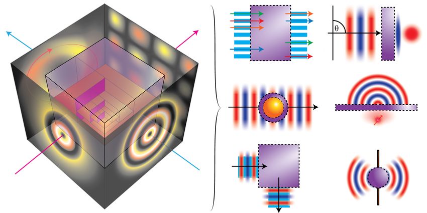
the development of a variety of limits on communication FIG. 1. Investigation schematic and sample applica-
tions. The figure sketches the central question explored in
in general quantum systems, e.g. Refs. [4–7]. Broadly,
this article: given a specified design volume(s) and mate-
even at the coarsest levels of physical description, there rial(s), how effectively can some particular collection of field
is generally some notion of invariants, and the existence transformations (described as input–output pairs) be real-
of such quantities implicitly precludes the possibility of ized? The panel on the left depicts an abstract optical de-
realizing complete engineering control. vice, the imitable black-box, converting a known set of input
Equating registers with electromagnetic fields and electromagnetic field profiles into a desired set of output field
scattering objects with channels [8], using the language profiles. The partitions interior to the design domain suggest
of communication theory, it is thus reasonable to assume how structural degrees of freedom or constraint clusters may
that there are certain channel-based limits on the extent be refined to improve design performance and estimations of
that a collection of fields may be manipulated via mate- limit performance (bounds), respectively. The smaller images
to the right depict six (of the many) possible applications
rial structuring. The wave nature of Maxwell’s equations
that can be easily described within this framework. Working
sets a fundamental relation between wavelength and fre- from left-to-right, top-to-bottom, theses illustrations repre-
quency (for propagation) that cannot be arbitrarily al- sent a spatial multiplexer, a metaoptic lens, a cloaking shell
tered by any realizable combination of material and ge- for an enclosed object, a light extractor (enhancing radiative
ometry. Consequently, the scattered fields generated by emission from a dipolar source), a waveguide bend, and a
any true object cannot be matched to any freely selected directional antenna.
magnitude and phase profile, and so, certain transforma-
tions cannot be achieved with perfect fidelity (e.g. known
limits on light trapping [9–11], cloaking bandwidths [12– tiplexing [22–24] and computing [25–27], the important
14], delay-bandwidth products [15–17], etc.) question is not whether such fundamental limitations ex-
However, in establishing a means of evaluating the ist, but rather what quantitative implications can be de-
potential of present and future electromagnetic devices duced in a given setting. Beyond well established con-
to address challenges requiring complex functionalities, siderations like the need to conserve power in passive
such as artificial neural networks [18–21], spatial mul- systems and the classical diffraction limit of vacuum [28],
such specific channel features are typically unknown [29].
Moreover, it is seldom clear what level of possible per-
formance improvement could be sensibly supposed, even
∗ Equal contribution to within multiple orders of magnitude [30–32]. Archi-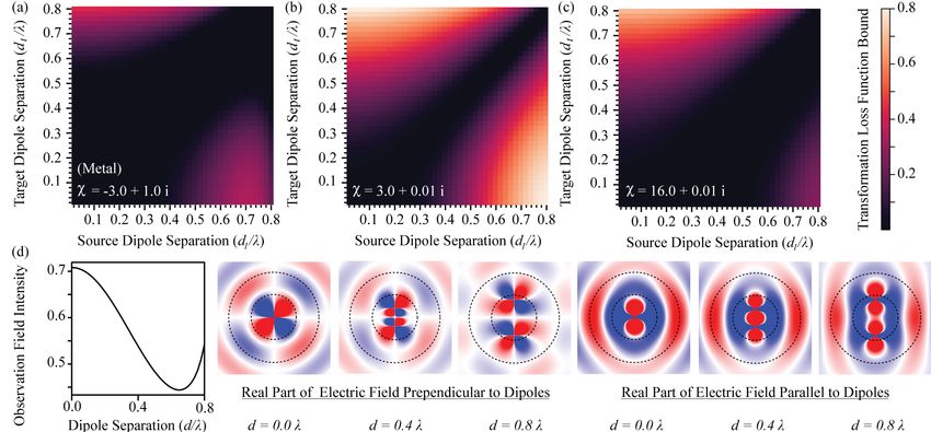
2

tectures possessing impressive field-transformation capa-       in Sec. III, tied to the ability of the formulation to enforce
bilities have already been demonstrated, from free-space        that all channel functionalities map to a unique (single)
(grating) couplers [33, 34] to beam steering [35, 36] and       optimal geometry.
polarization control [37, 38], suggesting that large-scale
optimization methods may allow scattering attributes to
be tailored to a far greater degree than what has been                I.   CHANNEL LIMITS IN PRIOR ART
seen in past intuition-based designs. Simultaneously,
ramifying from the core ideas of Lagrange duality and in-          Excluding techniques based on Lagrange duality to
terpreting physical relations as optimization constraints       constrain electromagnetic design objectives, which are
expounded below [39–42], a string of recent articles on         covered in greater detail in Sec. II, three major threads
improved bounds for scattering phenomena (including ra-         studied in prior art have substantially informed the find-
diative heat transfer [32], absorbed power [43], scattered      ings and discussion below.
power [44], and Purcell enhancement [45]) have shown               Decomposition—Any finite dimensional linear opera-
that, in some cases, only modest improvements over stan-        tor (or more generally any compact operator such as the
dard designs are even hypothetically attainable [44–53].        scattering T operator of electromagnetism) has a corre-
   In this article, we demonstrate that this rapidly devel-     sponding singular value decomposition [54]. For almost
oping program for calculating bounds on scattering phe-         any example of practical interest, particularly those with
nomena can be applied to determine limits on the accu-          discrete representations, there are hence corresponding
racy to which any particular set of field transformations       notions of rank and pseudo rank [8, 55–58].
may be implemented, providing an initial exploration of            Rank —Potential field transformations between collec-
channel characteristics in the context of classical elec-       tions of registers are inherently limited by any bounds
tromagnetic (multi-wavelength and multi-port) devices.          on maximal rank or pseudo rank. Any set of channels
The article is broken into three sections. In Sec I, a con-     connecting registers that do not overlap in space is in-
densed overview of related work examining channel limits        herently limited by the rank (pseudo rank) of its as-
on electromagnetic devices prior to the articles referenced     sociated free propagation operators (the Green’s func-
above is provided. Section II then summarizes the guid-         tion) [30, 44, 59, 60].
ing optimization outlook of the rest of the article along          Size—The rank (pseudo rank) characteristics of free
with current methods for constructing T-operator (scat-         propagation in electromagnetics depend explicitly on ge-
tering theoretic) bounds. During this brief overview, two       ometry. That is, there are cases where possible field
innovations necessary for handling generic input–output         transformations are strongly limited by the spatial vol-
formulations are introduced: a further generalization on        ume occupied by the registers [43, 59].
the variety of operator constraints that can be imposed            The main difference between past studies of channel
based on the definition of the T operator, beyond the           limits utilizing these ideas and the T-operator approach
possibility of local clusters examined in Refs. [45, 51, 52],   given in Sec. II lies in the incorporation of additional
and a generalization of the type of vector image con-           physical constraints concerning the generation of polar-
straints that should be usually considered, as required         ization currents (within a scattering object) in order to
to enforce that every transformation in an input–output         effect a desired transformation. More concretely, it is
set references the same underlying structure. Finally,          often possible to abstractly describe a device in terms
Sec. III provides a number of exemplary applications of         of (possibly intersecting) design and observation regions.
the theory, including studies of model computational ker-       Taking a simplistic description of a near-field microscope
nels, domain shielding and near-field focusing. For the         as an example, the magnifying lens may be thought of
chosen loss function (the quadratic distance or two-norm        as a design volume, and the final connection between the
between the set of desired target and realizable fields),       optical components and the electro–optic readout as an
the gap between calculated bounds and the performance           observation region. (As seen in Fig. 2, the design and
of device geometries discovered via topology (or “den-          observation regions are closely linked to the sender and
sity”) optimization is regularly found to be of unit order.     receiver registers in optical communication.) Under this
The observed trade-offs between the size of the design do-      regional decomposition, the end goal of various applica-
main, the supposed material response of the device, the         tions can be understood as minimizing the power differ-
specific transformations (channels) considered, the num-        ence between the true total field created in the observa-
ber of constraint clusters, and the calculated limits reveal    tion region ( Eto ) [42], resulting from a known incident
several intuitive trends. Most notably, achievable perfor-      field ( Ei ), and a given target output ( Eo ):
mance is strongly dependent on the nature and num-
ber of communication channels, with larger device sizes                          min|Jg i k Eto − Eo k22 .               (1)
                                                                                      d
and indices of refraction resulting in greater achievable
spatial resolution and transformations, in line with prior      (Here, subscripts mark domains of definitions and super-
heuristics [REF]. For the wavelength-scale systems in-          scripts label different types of fields.) Supposing that po-
vestigated here, the variability in achievable performance      larizable media exists only within the design region (the
spans multiple orders of magnitude and, as demonstrated         device), following the notation of the upcoming section,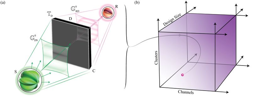
3

FIG. 2. Electromagnetic channel limits. (a) The properties of an electromagnetic channel(s) (C) depend on the environment
connecting a particular (collection of) sender (S) and receiver (R) register(s), including characteristics like the volume each
register occupies, their spatial separation, and the possibility of a transformation enabling polarizable device (D). Channel
limits in prior art have been formulated predominately by analyzing the individual operators describing each of these aspects in
isolation (e.g., the rank and pseudo rank of the free space Green’s function between the sender and receiver volumes G0RS ). Here,
in contrast, all environmental factors are treated simultaneously, accounting for the realities of interaction. (b) The difficulty
of attaining device performance bounds using the formulation presented in Sec. II, for some predefined material, depends
mainly on three variables: the number of regional constraints (spatial clusters) imposed, the number of channels (simultaneous
transformations) considered, and the physical volume of the design region. The way in which these attributes determine how
closely the computed bounds approximate achievable device performance is generally unknown and problem dependent. For
radiative thermal emission and integrated absorption, increasing domain size leads to increasingly tight bounds when only a
single constraint, the conservation of real power, is employed [43]. For radiative Purcell enhancement, recent results suggest
that predictive bounds for larger design domains require a larger number of constraints [45]. Additional regional constraints,
or concurrent analysis of additional channels, always produces tighter bounds.

in terms of the generated polarization field Jgd Eq. (1)           field transformations. Directly, without additional con-
becomes                                                            straints, the challenge associated with attaining a par-
                                  Z                                ticular polarization current |Jgd i within the design region
         min|Jg i k Eio − Eo + i G0od Jgd k22 .     (2)           cannot be inferred from Eq. (3). To include this infor-
              d                   ko
                                                                   mation into the minimization of Eq. (1), additional phys-
The minimum of Eq. (2) with respect to Jgd ,                       ical constraints must be taken into account. Achieving
                                                                   this aim, without making the resulting problem state-
         ko       †                       †
             G0od    Eo − Eio = G0od God Jgd , (3)                ment computationally infeasible, is precisely the goal of

      i
         Z                                                         the T-operator framework presented below.
illustrates the necessity of the three notions stated above.
First, even if Eq. (3) can be satisfied exactly, the mini-
mum of Eq. (1) may be nonzero if the span of the tar-                         II.   TECHNICAL DISCUSSION
get basis of G0od does not contain Eo − Eio . Second,
since in extending Eqs. (1)–(3) from single fields to col-          A.   Scattering theory, Lagrange duality, and limits
lections nothing in the form of the minimum solution is
altered, the rank (pseudo rank) of the Hermitian operator            Following the sketch provided in Ref. [29] (support-
      †
  G0od G0od sets a limit on the number of channels that            ing details can be found in Refs. [61–65]), there are two
can connect (interact) with any register contained in the          superficial distinctions that distinguish a scattering the-
observation domain. Third, as highlighted by the explicit          ory view of electromagnetics from Maxwell’s equations.
domain subscripts, the Green’s function (G0od ) connect-           First, supposing a local, linear scattering potential, the
ing the observation and design domains, on which the               fundamental wave relation from which all field properties
two previous points are based, depends on the geometric            are derived is
features of both regions.
                                                                                     Is = Is V−1 − G0 Ts ,

                                                                                                                           (4)
   While of obvious importance, it is clear that these ob-
servations do not fully encompass the difficulties associ-         where the s subscript denotes projection into the scat-
ated with the larger question of realizing a given set of          tering object, G0 is the background Green’s function of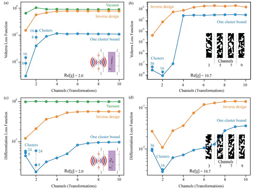
4

the design domain Ωs , throughout taken to be the vac-          is effectively a sesquilinear form on Ts .
uum Green’s function (truncated to a problem-specific                   X
                                                                             Ek Io Ek − 2 Re Ek Io Etk + Etk Io Etk
                                   2

volume) scaled by ko2 = (2π/λ) (so that all spatial di-         Obj =
mensions may be simply defined relative to the wave-                X
                                                                         k
length), V is the bulk (spatially local) scattering potential           Ek Io Ek − 2 Re            Ek Io Eik       + Eik Io Eik

                                                                =
of the material forming the design, I is the identity oper-         k
ator, and Ts is the scattering operator, formally defined
                                                                        + Eik T†s G0† Io G0 Ts + 2 Sym Io G0 Ts Eik

by Eq.(4) [66] [67]. (Although more general descriptions
                                                                        − 2 Re Ek Io G0 Ts Eik ,

are possible, it is implicitly assumed throughout this ar-                                                                            (7)
ticle that V = Iχ, where χ is electric susceptibility of
some isotropic medium.) Second, one of either the elec-         and the objective of the design amounts to a minimiza-
tromagnetic field or polarization field is singled out as       tion of
an initial [68], and all other fields are generated via the                 X
                                                                                Eik T†s G0† Io G0 Ts + 2 Sym Io G0 Ts Eik

                                                                Obj (Ts ) =
scattering operator Ts . This leads to a division of the
                                                                                k
theory into two classes: initial flux problems, where a
                                                                                                 Ek Io G0 Ts Eik

far-field incident flux Ei is assumed, generating a po-                             − 2 Re                                 .          (8)
larization current |Jg i = − (iko /Z) Ts Ei and scattered
                                                                Here, Sym [O] and Asym [O] denote symmetric (Her-
field Es = (iZ/ko ) G0 Jg , and initial source problems,        mitian) and anti-symmetric (skew-hermitian) parts of
where a polarization source Ji is assumed, generat-             O. (Other objective forms, e.g. originating from other
ing an electromagnetic field |Eg i = (iZ/ko ) G0 Ts V−1 Ji      norms, could also be considered, but (8) offers many use-
and total current Jt = Ts V−1 Ji .                              ful simplifications for both analysis and computation.)
                                                                Acting with T†s from the left on (4), giving T†s = T†s U† Ts
                                                                with U† = V−1 − G0 so that Asym [U] is positive definite,
   Given that most quantities related to power trans-           shows that the physical constraints of scattering theory
fer result from inner products between electromagnetic          can also be written as similar sesquilinear forms. As such,
and polarization fields [61], many common design objec-         any electromagnetic design objective of this input–output
tives within scattering theory, encompassing applications       form (Ref. [42]) can be cast as a quadratically constrained
varying from enhancing the amount of radiation that can         quadratic program [75, 76] (QCQP) by treating Ts as a
be extracted from a quantum emitter [69–71] to increas-         vector, i.e.
ing absorption into a photovoltaic cell [72–74], are given
by sesquilinear forms on the scattering operator Ts . As          min   Ts   Obj (Ts )
the central example investigated in this article, continu-
                                                                  such that (∀ l, m) Bl Ts Bm = Bl T†s UTs Bm ,
ing the discussion of Sec. I and covering all the specific
applications                                                                                                  (9)
           treated in Sec. III, suppose that a collection
of fluxes Eik , with k ranging over some finite indexing
                                                                over some basis [77] for the space of electromagnetic
set, is incident on a scattering design region Ω. Assume
                                                                fields over the design region Ωs . Although QCQP prob-
thatnthe goal
           o of the (input–output) device is to create a        lems are part of the non-deterministic polynomial-time
set Ek     of target fields within an observation region       (NP) hard complexity class, a number of relaxation tech-
Ωo , marked by a domain subscript o and spatial projec-         niques, as well as a range of well developed solvers,
tion operator Io , i.e. a collection of register mappings       are known to often yield accurate solution approxima-
 Eik 7→ Ek . Taking the Euclidean norm as a metric of          tions [78] (that may in fact be exact). Principally, let-
design performance,                                             ting L (Ts , λ) = Obj (Ts ) + λ C (Ts ) be the Lagrangian
                                                                of Eq. (9), with C (T) denoting the collection of imposed
                                                                scattering constraints and λ the associated set of La-
                                                                grange multipliers, it always possible to relax Eq. (9),
                                                                or any differentiable optimization problem for that mat-
         n         o n    o sX                                ter [79], to a convex problem by considering the uncon-
              Etk    , Ek                Etk − Ek k22 ,

  dist                       =   kIo
                                                                strained dual optimization problem
                                   k
                                                    (5)                                  maxλ G (λ) ,                                (10)
the equivalent objective (in the sense (5) and (6) have
the same minimum)                                               with G (λ) = minTs L (Ts , λ). Because any true solution
                                                                of Eq. (9) requires every constraint relation to be satis-
                                                                fied, for any collection of multipliers λ, G (λ) is always
                                                                smaller (resp. larger if the optimization objective is to
         n         o n    o X                                 maximize some quantity) than any solution of the primal
              Etk    , Ek             Etk − Ek k22 (6)        (original) optimization. Thus, in addition to providing a

 Obj                         = kIo
                               k                                means of obtaining approximate solutions to Eq. (9) [78],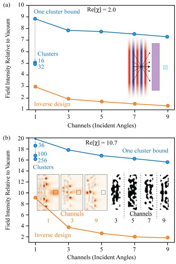
5
solving Eq. (10) also determines a bound, or limit, on refined mean-field approximations that mirrors the “bot-
the performance that could be possibly achieved by any tom up” optimization of a given objective with respect
realizable device geometry. By varying the constraints to structural degrees of freedom [80]. Letting |Ei de-
included in (9) these bounds can be tailored to encom- note some predefined electromagnetic flux, and making
pass select attributes of the channel(s) as one wishes, the simplifying choice that Mx = 1 for all x ∈ Ωc acting
such as qualifications on material composition (via V), on Eq. (13) with E . . . E gives
the available design domainn(via truncation
o of G0 ), and
the actual input fields (via Eik ). Further, although
Z Z
dx E∗ (x) · T (x) − dy T∗ (y) · U (y, x) · T (x)
we have not seriously examined the prospect, it is also
Ωc Ω
possible to apply similar reasoning to objective forms dif-
fering substantially from Eq. (6). = E PΩc T − T UPΩc T = 0, (14)
where the generated polarization current T is the image
B. Mean-field hierarchy (spatially localized of E under the action of Ts (Ts E 7→ T ). Returning
constraints) to Eq. (14), the selection of any cluster Ωc therefore de-
fines an averaging kernel for the scattering theory: over
Building on the above perspective, as described in Ωc the otherwise free field must respect the true physi-
greater detail in Refs. [45, 53], the T operator provides cal equations of electromagnetism, however, at any point
a natural means of obtaining arbitrarily accurate, con- x ∈ Ωc unphysical fluctuations of the field (deviations of
text specific, mean-field solution approximations. The the integrand from zero) are permitted [81].
operator relation given by Eq. (4) is equally valid under As any physical polarization current field Jg will au-
evaluation with any linear functional or vector, or com- tomatically satisfy any relation of the form of Eq. (14),
position with any other maps, and can hence be “coarse- any optimization that only imposes such relations over a
grained” (averaged). Expressly, to construct an appro- finite set of clusters {Pk } will automatically possess ob-
priate mean-field approximation, take PΩc to denote a jective values at least as optimal as what can be achieved
generalized spatial projection operator into the spatial if Eq. (4) is imposed in full. Hence, solving the mean-field
cluster (subregion) Ωc , with the added freedom that, at optimization
any point within Ωc , PΩc may transform the field in any
way. That is, taking the three dimensional nature of min / max |Ti Obj T
the electromagnetic and polarization vector fields into such that (∀ Ωk ) E PΩk T − T UPΩk T , (15)
account, PΩc may be any operator of the form
( similar to the mean-field theories used in statistical
0 x 6= y or x 6∈ Ωc physics [82, 83], game theory [84, 85] and machine-
PΩc (x, y) = , (11)
Mx x = y and x ∈ Ωc learning [86, 87], results in a bound (limit) on physically
realizable performance [88]. Due to the implicit wave-
where Mx , at any point in Ωc , is some any linear operator length scale contained in the Green’s function (G0 in U),
(3 × 3 matrix) on the three-dimensional vector space at there is, for most objectives, no meaningful difference
the point x. Recalling that Is is defined as between a mean-field fluctuating sufficiently rapidly and
( a physical field, satisfying Eq. (4) exactly. As a conse-
0 x 6= y or x 6∈ Ωs
Is (x, y) = , (12) quence, smaller clusters, effectively, lead to higher order
1 x = y and x ∈ Ωs mean-field theories that more closely bound what is actu-
ally possible. This tightening with decreasing cluster size
with 1 the identity operator (3 × 3 identity matrix), and
causes (15) to act as an intriguing complement to stan-
that the composition of any two spatial projections is
dard structural design. In “bottom-up” geometric opti-
equivalent to a single spatial projection into the intersec-
mization, the introduction of additional degrees of free-
tion of the two regions, any operator of the form given by
dom opens additional possibilities that improve achiev-
Eq. (11) commutes with Is , regardless of the actual ge-
able optima. In “top-down” mean-field optimization, the
ometry of the scatterer, allowing Eq. (4) to be rewritten
introduction of additional clusters results in additional
as
constraints that reduce the space of possibilities available
T†s P†Ωc Is = T†s P†Ωc Is V−1 − G0 Ts
to the design field T . Our present high-level approach
to solving Eq. (15) is described in Ref. [45].
⇒ T†s Is P†Ωc = T†s P†Ωc Is V−1 − G0 Ts
⇒ T†s P†Ωc = T†s P†Ωc V−1 − G0 Ts
C. Multiple transformations (channels)
⇒ PΩc Ts = T†s UPΩc Ts . (13)
Working with increasingly refined collections of clusters, When handling a collection of sources that span a rel-
sets of subdomains {Ωc } with c ranging over some index- atively small subspace, an efficient approach to comput-
ing set such that ∪c Ωc = Ω, Eq. (13) leads to increasingly ing T operator bounds through Eqs. 8 & 13 is to work6
with individual inputs and outputs. Take {|Sk i} to be main overarching features, which credibly apply beyond
a given collection of sources, and let {|Tk i} be the col- the actual scope studied, are seen. First, distinct chan-
lection of polarization fields resulting from the action of nels can display widely varying (often unintuitive) char-
Ts , Ts |Sk i 7→ |Tk i. Following Ref. [45], for any pair of acteristics. Second, both in terms of computed bounds
indices hk1 , k2 i, and each PΩc cluster operator, |Sk1 i and and the findings of inverse design, attainable performance
{|Tk1 i , |Tk2 i} must obey the relation may vary greatly as the number of channels increases—
the design freedom offered by spatial structuring in a
hSk1 | PΩc |Tk2 i = hTk1 | UPΩc |Tk2 i , (16) wavelength scale device is by no means inexhaustible.
Third, increasing the number of constraint clusters can
where, again, U = V−1† − G0† , and hF|Gi denotes the improve the accuracy of bounds calculations, but this
standard complex-conjugate inner product over the com- improvement is problem dependent and varies, in par-
R ∗
plete domain (hF|Gi = Ω dx F (x) · G (x) in the spatial ticular, with the material assumed. Throughout, as no
basis). In Eq.(16), the extension to pairs of sources and feature size can be imposed if one wishes to set bounds
polarization fields, compared to the single source con- on any possible geometry, quoted inverse design values
straints examined in Ref. [45], is necessary to account represent the performance of “grayscale” structures, al-
for the fact that a single scattering object (structured lowing each pixel to take on any susceptibility value of
media) simultaneously generates each |Tk i from each the form tχ with t ∈ [0, 1].
|Sk i. Over some set of clusters, using only the “diag-
onal” constraint between each source field (|Sk i) and
polarization response (|Tk i) is equivalent to considering A. Field screening
each source independently. But, by additionally includ-
ing “off-diagonal” interactions between pairs, Eq. (16) Objective—Minimize the spatially integrated field in-
introduces the requirement of a single consistently de- tensity over a subwavelength ball for two dipole fields,
fined scattering object. Supposing a spatial basis in the supposing that the distribution of scattering material (of
limit of “point” (vanishingly small) clusters and complete a predefined susceptibility) must be contained in a thin
field mixing, Eq. (16) becomes (∀ x ∈ Ω & hk1 , k2 i) surrounding shell.
The observation (shielded) region is taken to have a
S∗k1 (x) · Mx · Tk2 (x) radius of 0.2 λ, while the design domain is confined within
Z a shell of inner radius 0.2 λ and outer radius 0.24 λ. As
= dy T∗k1 (y) · U (y, x) · Mx · Tk2 (x) . (17) sketched in the inset of Fig. 3(a), the “separation vectors”
Ω
connecting the center of each dipole sources to the center
of the observation domain are supposed to be aligned.
Therefore, making use of the possible freedom in the def- The loss objective is defined as
inition of Mx , whenever any Tkn (x) is nonzero any of
the three local vector coordinates we must have kIobs Eta k22 + kIobs Etb k22
Loss Eta , Etb
= (20)
Z kIobs Eia k22 + kIobs Eib k22
Sk (x) = dy T∗k (y) · U (y, x) ,
∗
(18) with k. . .k2 denoting the Euclidean two-norm and Iobs
Ωs projection into the observation domain. Two clusters,
evenly dividing the radius of the design region (0.2 →
for all k and x ∈ Ωs , the collection of all spatial points 0.22 λ and 0.22 → 0.24 λ), are used in all bound compu-
in Ω where some Tk (x) 6= 0. Taking the adjoint, the tations.
totality of the point constraints given by Eq. (18) can be In the limit of large separation, the dipole fields within
codified as the design and observation domains closely resemble
−1 counter-propagating planewaves. Hence, the constant
|Tk i = U†Ωs |Sk i . (19) asymptote value seen as d approaches λ is, for all prac-
tical purposes, a bound on shielding for two opposing
Comparing with Eq. (4), Ωs thus determines the unique planewaves. The decrease of the bounds for small sep-
geometry of the scattering object (structured medium) aration, speculatively, is caused by a combination of lo-
for all sources. calization effects. As the dipoles are brought into the
near-field of the design, the bulk of the field magnitude
increasingly shifts towards the edge of the observation re-
III. APPLICATIONS gion. Consequently, inducing small shifts in the position
of the field results in a comparatively larger field expul-
In this section, the ideas presented in Sec. II are ap- sion. The presence of relatively larger evanescent fields
plied to several example applications, expounding the use likely also simplifies the suppression of total emission via
of input–output language to describe physical design as the (inverse) Purcell effect.
QCQP optimization problems, and demonstrating the The imposition of cross-constraints (solid lines), which
utility and tightness of the associated bounds. Three in the limit of point clusters enforce that all considered7
B. Dipole resolution and masking
Objective—Manipulate the field emanating from a pair
of axially aligned dipoles, again limiting the volume avail-
able for device design to a thin encompassing spherical
shell, so that exterior to the shell it appears that the
dipoles are separated by either a larger or smaller dis-
tance. If the field is altered so that the separation dis-
tance appears larger than it actually is, it is easier to
resolve that there are in fact two dipoles present, instead
of a single dipole of some effective strength.
More exactly, the input field is generated by a pair of
z polarized dipole sources, labeled 1 and 2, situated at
+di ẑ and −di ẑ for i = 1, 2, and the target field is taken to
arise from equivalent dipolar configuration with a distinct
separation, ±dt ẑ. The observation domain is set to be a
shell of half wavelength thickness enveloping the design
domain, which extends from an inner radius of 0.48 λ to
an outer radius of 0.5 λ. Bounds, in all cases, are com-
puted using ten spherical clusters, evenly spanning the
design domain with respect to radius. Additional techni-
cal details concerning the example are given in Sec. V A.
The bounds depicted in the three heat maps of Fig. 4,
exploring variations in both input d1 = d2 and output
dt pair separations, indicate that the challenge of ei-
ther reducing or enlarging the perceived separation of
the source varies sizably with supposed material prop-
erties and gap distances. For larger target or source
separations (dipoles approaching the interior surface of
the design domain) the increasingly dominant role of
evanescent fields makes almost any transformation chal-
lenging, especially in weakly polarizable media. Focusing
on Fig. 4(b), where the real part of the permittivity is
FIG. 3. Dipole screening and field transformations.
The figure depicts two representative three-dimensional ap-
limited to small positive numbers (weak dielectrics), the
plications of input–output bounds: limits on the ability of bounds prove that neither separation manipulation be-
any structured geometry confined to a thin shell to (a) screen havior is achievable in any practical sense when the input
dipole fields, and (b) mask the separation of dipole source and target separations vary by more than ≈ 0.25 λ. Con-
pairs within the encompassing environment. In both sit- versely, even under the imposition of considerably larger
uations, dashed lines mark independent bounds, calculated material loss (Im [χ]), panel (a) suggests that much better
without the inclusion of cross-constraints which enforce a performance is achievable with metals (Re [χ] < −1). In-
unique optimal structure across all field transformations, tuitively, the subwavelength characteristics of the system
while the solid lines result when source interactions effects do not preclude resonant response in this case since plas-
are taken into account. A material loss value of Im [χ] = 0.01 mon excitations remain possible. The observed asymme-
is assumed for all cases.
try between increasing and reducing perceived separation
seen in panels (b) and (c), which is largely absent in the
metallic example of panel (a), is likely also tied to decay-
ing waves: larger gaps produce larger evanescent fields
in the observation domain compared to what is provided
by the source, but smaller target separations do not.
channels are realized within one common geometry (see Figure 3(b) explores the impact of distinct source sep-
Sec. II C), is seen to produce a relatively small correction arations, varying d1 while keeping d2 = 0.7 λ fixed, for
to the bounds attained for independently optimized chan- a common target field corresponding to two co-located
nels (dashed lines). This suggests that although perfect dipoles at the center of the ball, dt = 0. The findings
shielding is not possible at sufficiently large dipole sepa- highlight the need to enforce that performance bounds for
ration, given the small shell and material constraints in- multiple channels refer to a unique scattering geometry,
vestigated, many structures may potentially achieve sim- achieved via the presence of cross-constraints in the opti-
ilar performance, i.e. the considered channels have yet mization (see Sec. II C). When the two channels are ana-
to “set” the scattering structure in any meaningful way. lyzed separately (dashed lines), the bound values match8
FIG. 4. Dipole resolution and masking. Considering the same three-dimensional system depicted in the inset of Fig. 3(b),
but with a single dipole-pair source, the three heat maps depict bounds on the ability of an arbitrary geometry made from
a specified material, restricted to a thin shell, to modify the perceived separation of a pair of axially aligned dipole sources,
as implied by the electric field exterior to the design. Setup details are given in the main text. In moving from the trivial
diagonal (no transformation) to the top left, the target field is set to be the field of an axial dipole pair further separated than
that of the source. Opposingly, in moving to the bottom right, the target field is set to be the field of an axial dipole pair less
separated than that of the source. The observed asymmetry between these two directions provides evidence of the ostensibly
greater challenge of resolving closely separated fields, compared to masking separation. Field profiles for representative dipole
pairs, along with the average field intensity within the observation domain (dashed lines), are given in panel (d).
those displayed on the heat maps of Fig. 4, with the (thickness) of 0.5 λ and parallel length of 2 λ, insets
contribution of source 1 to the loss function approach- Fig. 5(a) and Fig. 5(c). The input observation plane
ing zero as d1 → 0, since in this regime the source and is set at distance of 0.25 λ from the input edge of the
target fields match. However, when cross-constraints are design region, and the output observation plane is lo-
included, the lack of a need for a design in this regime cated at a distance of 0.25 λ from the output edge of
for the first source is at odds with what is needed to con- the design region. Incident fields are generated by dipole
vert the field of the widely separated d2 source, leading to (pixel) sources placed on a source plane, running paral-
degraded performance. As d1 approaches d2 , the require- lel to the long edge of the design region, situated at a
ment of a unique gemometry no longer introduces addi- distance 0.2 λ from the input observation plane. The
tional requirements, and thus the “simultaneous” (cross- source plane has length of 1.5 λ and is centered in rela-
constrained) and “independent” results merge. tion to the design domain, creating a 0.25 λ offset from
the top and bottom edges of the design region and in-
put and output planes. For the Volterra operator, the
target fields along the output plane, letting y denote the
C. Math kernels (integration and differentiation)
direction running parallel to the long edge
R y of the design
region, are calculated as E (x , y) = 0 dy 0 Ei (xi , y 0 ),
Objective—Within a bounding rectangle, design a two- with x and xi denoting the common coordinate of the
dimensional scattering profile, for a known collection of output and input plane, respectively. For the differ-
incident waves, such that the relation between each inci- ential operator, keeping the above notation, the target
dent field and total field, along specified input and out- fields are calculated as E (x , y) = ∂Ei (xi , y) /∂y, im-
put observation planes, reproduces the action of Volterra plemented as a finite-difference approximation on a com-
(integration) or differentiation operator. Given that the putational grid. The optimization objective is defined
Volterra and differentiation kernels are two of the basic by Eq. (7) and the bounds formulated following the de-
elements of differential equations, these examples are of scription given in Sec. II. Further implementation details
considerable interest in relation to recent proposals for appear in Sec. V B. The loss function values appearing in
optical computing [25–27].
The design region is chosen to have a transverse length9
FIG. 5. Volterra and differentiation kernels. Following the description in the main text, the figure depicts limits on
the degree to which a structured medium of a given electric susceptibility χ, confined to a rectangular design domain, may
implement Volterra (top row) and differentiation (bottom row) kernels, as as function of the size of the subbasis (number of
channels or transformations) over which the operator is defined. The cluster labels reference the number of cluster constraints
imposed on the design domain, following the discussion of Sec. II and with further details given in the main text. Notably,
the calculated bounds generally agree to within an order of magnitude of the performance of inverse designed structures when
either the rank of the specified subbasis, or number of imposed clusters, is large. In all four cases, a material loss value of
Im [χ] = 0.01 is assumed. Representative topology-optimized structures are included as insets in (b) and (d). The performance
of these binarized systems is roughly a factor of two worse than the associated “grayscale” geometries compared to in the figure.
Fig. 5 are determined by The most striking aspect of the findings displayed in
Fig. 5, especially when viewed in conjunction with Fig. 6,
kIout Et − E k22 is the widely varying characteristics observed between
t
Loss E = . (21) the four cases. For the Volterra and differentiation ker-
kIout Ei k22 + kIout E k22 nels, at least within the subbasis used here, the num-
In Eq. (21), Iout denotes projection onto the output ob- ber of channels considered has a remarkable influence on
servation plane, and an overline on a vector indicates the observed limit values. Given that analogous trends
vertical concatenation over all likenamed fields indexed are seen in performance of the associated structural opti-
by the incident waves, i.e. Et = Et1 , . . . , EtN for
mizations, it can be safely concluded that this behavior is
N sources. The cluster numbers appearing in Fig. 5 re- fundamental, hinting that there is a sort of Fourier (res-
fer to specific, even and consistent, divisions of the design olution) limit at play (e.g., size-dependent constraints on
domain rectangle along its long and short edges. Writing space-bandwidth products are known to limit the degree
division of the short edge first, 8 = 2 × 4, 16 = 2 × 8, to which a given optical feature may be resolved with a
24 = 3 × 8 and 36 = 3 × 12. finite device [89, 90]). Moreover, presumably because dif-10
ferentiation demands creation of more rapid profile varia-
tions whereas Volterra operations demand only smooth-
ing, loss function values (for both bounds and inverse
design) differ by multiple orders of magnitude for small
numbers of channels (≈ 3) before reaching “asymptotes”
that differ roughly by a factor of 10, for χ = 10.7+i 0.01.
Conversely, in the focusing example examined in Fig. 6,
the bounds exhibit only a weak dependence on the num-
ber of channels in either representative material. While
a precise account of the factors leading to these differ-
ences is likely challenging, it should be noted that in all
cases the objective is bounded (from above or below)
by performance that could be achieved in vacuum or a
full slab, and so the appearance of plateaus when per-
formance is poor should come as no surprise. A related,
albeit more intuitive, dichotomy is seen with respect to
the number of clusters imposed and the magnitude of
electric susceptibility (Re [χ]). For Re [χ] = 2, subdivid-
ing the domain generally leads to substantial tightening,
while for Re [χ] = 10 many more clusters are needed to
produce meaningful alterations owing to the decrease in
the effective wavelength in the medium.
D. Near-field lens (metaoptics)
Objective—Working within a given bounding rectan-
gular design domain, maximize the average field inten-
sity within a specified focal region for a predefined set of
incident plane waves spanning a cone of incidence.
The size of the rectangular design region is character-
ized by the lengths Ld1 = 0.5 λ and Ld2 = 2 λ, inset Fig. 6.
The focal region is a square centered along Ld2 , with side
length Lf1 = Lf2 = 0.25 λ. The middle of the focal region FIG. 6. Focusing metalens. Highlighting the applicabil-
is set to reside at a distance of 0.5 λ from the outgoing ity of the proposed method to establish limits on metaoptical
elements, the figure provides bounds on the ability of any
edge of design region. The design objective is
structure confined within a rectangular domain of subwave-
n o N length thickness to enhance the average field intensity over
a predefined focal region in the near field of the structure,
X
Obj Etk = max Eti Ifocal Eti (22)
for a given collection of incident planewaves. Also shown are
i=1
comparative performances of inverse designed structures. A
where the summation index runs over the N angles of material loss value of Im [χ] = 0.01 is supposed in all cases.
incidence, evenly distributed over a cone of (N − 1) × 15◦ Binarized structures for 3, 5, 7 and 9 channels, producing rel-
ative field-enhancement factors of 5.27, 2.66, 2.56 and 1.64
degrees centered on the midpoint of L2d . As before, the
respectively, are included as insets. Quoted values for the
cluster labels given in Fig. 6 reference even divisions of inverse design curve correspond to “grayscale” structures.
the rectangular design domain along its short and long
edges: 16 = 2 × 8, 32 = 4 × 8, 36 = 3 × 12, 100 = 5 × 20,
and 256 = 8 × 32.
Even in comparison to previous examples, the extent to largely responsible for these findings. First, the focusing
which inverse design is able to approach the limit values problem does not impose any specific target profile for
produced by the formulation of Sec. II is notable. For a the output fields, inset Fig. 6(b), leading to a greater va-
single source (a normally incident planewave), agreement riety of geometric possibilities with similar focusing per-
within a factor of 3 is achieved when a single cluster con- formance. Second, given the assumed design domain, the
straint is supposed, and as increasingly localized domain specified location and volume of the focal region makes
constraints are imposed the performance gap is seen to the problem more difficult than what might be naively
nearly close. Hence, somewhat surprisingly, the relatively expected [91]; quite different results may be encountered
poor field localization values achieved by the topology if the “spot size”, or separation between the focus and
optimized (inverse design) geometries are in fact not far design domain, are reduced. Third, the extended nature
from ideal. We suspect that three underlying factors are of planewave sources naturally suggests the uniform clus-11
ter constraints that have been employed. Contrastingly, whether some reasonably good approximation can actu-
for the Volterra and difference kernels, it is plausible that ally be solved in an acceptable amount of time. With
non-uniform cluster distributions, or simply smaller clus- this in mind, we believe that the results presented above
ters, could lead to tighter bounds. A systematic study of provide substantial reason for optimism.
such questions, once a more resource-effective approach Finally, the specificity of the program presented in the
for solving Eq. (9) is found [53], remains as an important main text raises a prescient question pertaining to re-
direction for future work. alizing abstract transformations. Expressly, there are
many instances in which the primary concern is how well
the transformation can be implemented between a given
number of undetermined inputs and outputs (channels).
IV. SUMMARY DISCUSSION The distinction amounts, in essence, to the same shift in
perspective advocated for in recent “end-to-end” inverse
design formulations [95, 101] and waveform optimization
In summary, we have shown that recently developed investigations [102, 103]: the exact characteristics of the
methods for calculating limits on sesquilinear electromag- domain and codomain sets for some particular discrim-
netic objectives [42, 45, 51–53], can be applied to a wide ination or transformation are often mutable, and only
variety of design problems, including spatial multiplex- important in so far as they implicitly alter achievable
ing [22–24], metaoptics [92–95], linear computation [25– performance. The duality program outlined above can
27] and light extraction [96–99]. Employing the lan- be extended to treat this problem in a variety of ways,
guage of communication theory, this program stands as and we intended to present this analysis in detail in an
a significant extension of prior work on channel-based upcoming work.
electromagnetic limits [8, 30, 55–60]. Namely, although
highly insightful, the characteristics of the background
Green’s function connecting the volumes containing par- ACKNOWLEDGMENTS
ticular sender and receiver registers are generally insuffi-
cient for accurately assessing whether the extent to which
This work was supported by the National Science
some desired communication can occur, particularly in
Foundation under the Emerging Frontiers in Research
wavelength-scale devices. Rather, as may be confirmed
and Innovation (EFRI) program, EFMA-1640986, the
by a survey of the results presented in Sec. III, the degree
Cornell Center for Materials Research (MRSEC) through
to which communication between a predefined collection
award DMR-1719875, and the Defense Advanced Re-
of registers can occur may depend strongly on a range of
search Projects Agency (DARPA) under agreements
other environmental factors, such as the physical size and
HR00112090011, HR00111820046 and HR0011047197.
response parameters available for designing the channels,
The views, opinions and findings expressed herein are
and the spatial profile of the register fields.
those of the authors and should not be interpreted as
The strong correspondence observed between bounds representing official views or policies of any institution.
computed with this approach and the findings of in-
verse design exemplified in Sec. III continues many of
the trends seen in the earlier works cited above. Regard- V. APPENDIX
less of the particular objective and distribution of cluster
constraints considered, we have yet to encounter a sit- A. Off-origin dipole spherical wave expansions
uation in which strong duality does not hold [100]. As
such, it would seem that the outstanding difficulties of
Following results of Ref. [104], as explained in Refs. [64,
constructing a general toolbox for realizing (tight) limits
105], off-origin, on-axis, outgoing spherical waves can
that incorporate the full wave physics and limitations of
be expanded in terms of on-origin outgoing and regular
Maxwell’s equations, and in turn offer guidance for prac-
spherical waves as
tical designs, are computational [29, 45, 53]. All present
evidence indicates that optimization problems following P
in± reg
the form of Eq. (15) can be solved exactly via the duality 0 0 Up0 p,l0 lm (d) Wp0 l0 m (r ± dẑ) r < d
out p ,l
relaxation described in Sec. II. If this is indeed the case, Wplm (r) = P out± out ,
0 0 Up0 p,l0 lm (d) Wp0 l0 m (r ± dẑ) r > d
then the matter of central importance is not whether p ,l
there is some configuration of clusters that will capture (23)
all key effects that physically limit communication, but where12
X l(l + 1) + l0 (l0 + 1) − ν(ν + 1)
Upin±
0 p,l0 lm (d) = δpp0 ∓ i mdko (1 − δpp0 ) Ah±
l0 lνm (d), (24)
ν
2
X l(l + 1) + l0 (l0 + 1) − ν(ν + 1)
Upout±
0 p,l0 lm (d) = δpp0 ∓ i mdko (1 − δpp0 ) Aj±
l0 lνm (d), (25)
ν
2
s
(2l + 1)(2l0 + 1) l l0 ν l l0 ν
m l−l0 ±ν
Ah±
l0 lνm (d) = (−1) i (2ν + 1) hν (dko ) , (26)
m −m 0
l(l + 1)l0 (l0 + 1) 0 0 0
s
(2l + 1)(2l0 + 1) l l0 ν l l0 ν
j± m l−l0 ±ν
Al0 lνm (d) = (−1) i (2ν + 1) j (dko ) . (27)
l(l + 1)l0 (l0 + 1) 0 0 0 m −m 0 ν
In Eqs. (24)–(27), the large round brackets are Wigner- summation limits are set by explicit evaluation of the
3j symbols, jν and hν denote the spherical Bessel and Wigner-3j selection rules and
Hankel functions of the first kind respectively, and the s
plus and minus signs indicate the sign of the necessary ν 2 + l(l + 1) − ν(ν + 1) 1−ν−l 6l + 3
Ll = (2ν + 1) i .
coordinate transformation. Noting that the field of a ẑ- 2 2l(l + 1)
polarized dipole radiation consists entirely of the N1,0 (33)
outgoing wave,
iko B. Computation for two-dimensional examples
Ez (r, θ, φ) = √ N1,0 (r, θ, φ) , (28)
6π
The Green’s function representations used for com-
the field of an off-axis dipole can thus be computed from
puting bounds in all two-dimensional examples were ob-
Eqs. (24)–(27) by setting p = N, l = 1, and m = 0
tained by the open-source ceviche FDFD package [106].
implying, through the Wigner selection rules that the
The basis used for representing fields in all such cases are
on-origin regular M waves, RgM, waves need not be in-
the individual discretization pixels of the FDFD compu-
cluded. Using this knowledge, the expansion coefficients
tation. Correspondingly, the matrix representation of the
for an off-origin, on-axis, dipole can be reduce to
Green’s function connects every pixel with a numeric ap-
iko proximation of the field generated by a dipole source at
Ez−dẑ (r) = √ N1,0 (r + dẑ) the location of the pixel.
6π For all studies with a free space background, the trans-
iko P∞
( in−
l=1 UN N,l,1,0 RgNl,0 (r) (r < d) ,
√ lational invariance of the Maxwell is exploited to con-
= ik6π P∞ out− struct the matrix representation of the Green’s function
l=1 UN N,l,1,0 Nl,0 (r) (r > d) ,
√o
6π
from a single dipole field solve. Concretely, consider a do-
(29)
main of shape (Nx , Ny ) in pixels. The required represen-
ik o tation of G0 is then a square matrix of dimension Nx Ny ,
Ez+dẑ (r) = √ N1,0 (r − dẑ)
6π where the j-th column is the field created by an electric
iko P∞ dipole at position j. This matrix can be obtained in a
( in+
l=1 UN N,l,1,0 RgNl,0 (r) (r < d) ,
√
= ik6π P∞ out+ single solve by placing a dipole at the center of a larger
l=1 UN N,l,1,0 Nl,0 (r) (r > d) ,
√o
6π (2Nx − 1, 2Ny − 1) domain and observing the calculated
(30) field in sliding a window of size (Nx , Ny ).
To account for the cross-source constraints in the pres-
where ence of multiple sources, compared to the approaches we
l+1 2 have used in prior works [45], the fields and matrices for
in−
X 1 l ν each of the individual sources are grouped into “super”
UN N,l,1,0 = Lνl hν (dko ) , (31)
0 0 0 vectors and matrices:
ν=l−1
l+1 2 T1 ZT1 T1 . . . ZT1 TN
X 1 l ν
T = ... ZT T = ... .. (34)
in+
UN N,l,1,0 = (−1)ν Lνl hν (dko ) . (32) ..
.
0 0 0 .
ν=l−1
TN ZTN T1 . . . ZTN TN
out− out+
UN N,l,1,0 and UN N,l,1,0 are equivalently defined but with As such, the dimension of the vectors and matrices in-
the Hankel functions of the first kind, hν (dko ), replaced volved in the calculation of a N -source bound scales lin-
by Bessel functions of the first kind. In these expressions, early with N . To facilitate computation of bounds for13
large device footprints and values of N , an Arnoldi basis respect to B̄0 , . . . , B̄i−1 , giving B̄i . The partial basis for
for U is computed to more efficiently represent the |Ti the generated block Krylov subspace at the end of the
image field. For any given problem, the only vectors that i-th iteration is the thus the aggregate of all the column
interact with the primal degrees of freedom, Tn , are vectors of B̄0 , . . . , B̄i . Denoting U restricted to the i-th
the sources, Ein , and the linear coefficients of Tn Krylov subspace as Ui , the representation is effectively
in the primal objective Onlin . Hence, these vectors complete when the column norms of U−1 i B̄0 converge to
within a certain tolerance, Ref. [29].
Ei1 EiN
B0 = ... O1lin ... O1lin , (35)
Inverse design results for all two dimensional examples
posses favorable convergence characteristic for computing are also computed using ceviche using a standard topol-
the dual via Arnoldi iterations. For communications type ogy optimization [91]. For sake of comparison with the
problems Onlin = G†od En − Ein , while for the met-
optimization problem underlying the bound formulation,
alens problem Onlin = G†od Ein . To begin the Arnoldi grayscale structures are treated as viable. That is, in any
procedure, B0 is orthonormalized to give B̄0 . The i-th particular design, the permittivity value of a given pixel
iteration is then computed by generating Bi = UB̄i−1 , can take any value in the convex set bounded by 0 and
and then orthonormalizing Bi both internally and with the quoted material value.
[1] Sergio Verdu. Fifty years of Shannon theory. IEEE passive quasistatic cloaking. Journal of Mathematical
Transactions on information theory, 44(6):2057–2078, Physics, 58(7):071504, 2017.
1998. [15] H. John Caulfield and Tomas Hirschfeld. Optical com-
[2] Pierre-Marie Robitaille. Kirchhoff’s law of thermal munication at the source bandwidth limit. Applied Op-
emission: 150 years. Progress in Physics, 4:3–13, 2009. tics, 16(5):1184–1186, 1977.
[3] Claude E Shannon. A mathematical theory of com- [16] Kosmas L Tsakmakidis, Linfang Shen, Sebastian A
munication. The Bell System Technical Journal, 27(3): Schulz, Xiaodong Zheng, John Upham, Xiaohua Deng,
379–423, 1948. Hatice Altug, Alexander F Vakakis, and Robert W
[4] John Brian Pendry. Quantum limits to the flow of in- Boyd. Breaking lorentz reciprocity to overcome the
formation and entropy. Journal of Physics A: Mathe- time-bandwidth limit in physics and engineering. Sci-
matical and General, 16(10):2161, 1983. ence, 356(6344):1260–1264, 2017.
[5] Carlton M Caves and Peter D Drummond. Quantum [17] Sander A Mann, Dimitrios L Sounas, and Andrea Alù.
limits on bosonic communication rates. Reviews of Mod- Nonreciprocal cavities and the time–bandwidth limit.
ern Physics, 66(2):481, 1994. Optica, 6(1):104–110, 2019.
[6] Michal Horodecki, Pawel Horodecki, and Ryszard [18] Yaser S Abu-Mostafa and Demetri Psaltis. Optical neu-
Horodecki. Limits for entanglement measures. Phys- ral computers. Scientific American, 256(3):88–95, 1987.
ical Review Letters, 84(9):2014, 2000. [19] Tyler W Hughes, Ian AD Williamson, Momchil Minkov,
[7] Stefano Pirandola, Riccardo Laurenza, Carlo Ottaviani, and Shanhui Fan. Wave physics as an analog recurrent
and Leonardo Banchi. Fundamental limits of repeater- neural network. Science advances, 5(12):eaay6946, 2019.
less quantum communications. Nature communications, [20] Ying Zuo, Bohan Li, Yujun Zhao, Yue Jiang, You-
8(1):1–15, 2017. Chiuan Chen, Peng Chen, Gyu-Boong Jo, Junwei Liu,
[8] David AB Miller. Waves, modes, communications, and and Shengwang Du. All-optical neural network with
optics: a tutorial. Advances in Optics and Photonics, nonlinear activation functions. Optica, 6(9):1132–1137,
11(3):679–825, 2019. 2019.
[9] Eli Yablonovitch. Statistical ray optics. Journal of the [21] Wim Bogaerts, Daniel Pérez, José Capmany, David AB
Optical Society of America, 72(7):899–907, 1982. Miller, Joyce Poon, Dirk Englund, Francesco
[10] Dennis M Callahan, Jeremy N Munday, and Harry A Morichetti, and Andrea Melloni. Programmable
Atwater. Solar cell light trapping beyond the ray optic photonic circuits. Nature, 586(7828):207–216, 2020.
limit. Nano letters, 12(1):214–218, 2012. [22] David J Richardson, John M Fini, and Lynn E Nel-
[11] Andrey E Miroshnichenko and Michael I Tribelsky. Ul- son. Space-division multiplexing in optical fibres. Na-
timate absorption in light scattering by a finite obstacle. ture Photonics, 7(5):354–362, 2013.
Physical Review Letters, 120(3):033902, 2018. [23] Juhao Li, Fang Ren, Tao Hu, Zhengbin Li, Yongqi
[12] Hila Hashemi, Baile Zhang, John D Joannopoulos, and He, Zhangyuan Chen, Qi Mo, and Guifang Li. Re-
Steven G Johnson. Delay-bandwidth and delay-loss lim- cent progress in mode-division multiplexed passive op-
itations for cloaking of large objects. Physical Review tical networks with low modal crosstalk. Optical Fiber
Letters, 104(25):253903, 2010. Technology, 35:28–36, 2017.
[13] Francesco Monticone and Andrea Alù. Invisibility ex- [24] Zhenshan Yang, Xiaoguang Zhang, Bin Zhang, Xia
posed: physical bounds on passive cloaking. Optica, 3 Zhang, Zhentao Zhang, Xiangguo Meng, and Chenglin
(7):718–724, 2016. Bai. Density-matrix formalism for modal coupling and
[14] Maxence Cassier and Graeme W Milton. Bounds on dispersion in mode-division multiplexing communica-
herglotz functions and fundamental limits of broadband tions systems. Optics Express, 28(13):18658–18680,You can also read