The Completed SDSS-IV extended Baryon Oscillation Spectroscopic Survey: Large-scale Structure Catalogs for Cosmological Analysis
←
→
Page content transcription
If your browser does not render page correctly, please read the page content below
SDSS DR16 LSS Catalogs   1

                                               The Completed SDSS-IV extended Baryon Oscillation Spectroscopic
                                               Survey: Large-scale Structure Catalogs for Cosmological Analysis

                                               Ashley J. Ross1? , Julian Bautista2 , Rita Tojeiro3 , Shadab Alam4 , Stephen Bailey5 ,
                                               Etienne Burtin6 , Johan Comparat7 , Kyle S. Dawson8 , Arnaud de Mattia6 , Hélion
                                               du Mas des Bourboux8 , Héctor Gil-Marı́n9,10 , Jiamin Hou7 , Hui Kong1 , Brad W.
                                               Lyke11 , Faizan G. Mohammad12,13 , John Moustakas14 , Eva-Maria Mueller2 , Adam
                                               D. Myers11 , Will J. Percival12,13,15 , Anand Raichoor16 , Mehdi Rezaie17 , Hee-Jong
                                               Seo17 , Alex Smith6 , Jeremy L. Tinker18 , Pauline Zarrouk19,6 , Cheng Zhao16 , Gong-
arXiv:2007.09000v1 [astro-ph.CO] 17 Jul 2020

                                               Bo Zhao20,21 , Dmitry Bizyaev22 , Jonathan Brinkmann22 , Joel R. Brownstein8 , Aure-
                                               lio Carnero Rosell23 , Solène Chabanier6 , Peter D. Choi24 , Chia-Hsun Chuang25 , Irene
                                               Cruz-Gonzalez26 , Axel de la Macorra26 , Sylvain de la Torre27 , Stephanie Escoffier28 ,
                                               Sebastien Fromenteau29 , Alexandra Higley11 , Eric Jullo27 , Jean-Paul Kneib16 , Jacob
                                               N. McLane11 , Andrea Muñoz-Gutiérrez26 , Richard Neveux6 , Jeffrey A. Newman30 ,
                                               Christian Nitschelm31 , Nathalie Palanque-Delabrouille6 , Romain Paviot27 , Anthony R.
                                               Pullen18,32 , Graziano Rossi24 , Vanina Ruhlmann-Kleider6 , Donald P. Schneider33,34 ,
                                               Mariana Vargas Magaña26 , M. Vivek33,35 , Yucheng Zhang18
                                               1
                                                 Center for Cosmology and Astro-Particle Physics, Ohio State University, Columbus, Ohio, USA
                                               2
                                                 Institute of Cosmology & Gravitation, Dennis Sciama Building, University of Portsmouth, Portsmouth, PO1 3FX, UK
                                               3
                                                 School of Physics and Astronomy, University of St Andrews, St Andrews, KY16 9SS, UK
                                               4
                                                 Institute for Astronomy, University of Edinburgh, Royal Observatory, Edinburgh, EH9 3HJ, UK
                                               5
                                                 Lawrence Berkeley National Laboratory, 1 Cyclotron Road, Berkeley, CA 94720, USA
                                               6
                                                 IRFU,CEA, Université Paris-Saclay, F-91191 Gif-sur-Yvette, France
                                               7
                                                 Max-Planck-Institut für Extraterrestrische Physik, Postfach 1312, Giessenbachstr., 85748 Garching bei München, Germany
                                               8
                                                 Department Physics and Astronomy, University of Utah, 115 S 1400 E, Salt Lake City, UT 84112, USA
                                               9
                                                 Institut de Ciències del Cosmos, Universitat de Barcelona, ICCUB, Martı́ i Franquès 1, E08028 Barcelona, Spain
                                               10
                                                  Institut dEstudis Espacials de Catalunya (IEEC), E08034 Barcelona, Spain
                                               11
                                                  Department of Physics and Astronomy, University of Wyoming, Laramie, WY 82071, USA
                                               12
                                                  Waterloo Centre for Astrophysics, Department of Physics and Astronomy, University of Waterloo, Waterloo, ON N2L 3G1, Canada
                                               13
                                                  Department of Physics and Astronomy, University of Waterloo, Waterloo, ON N2L 3G1, Canada
                                               14
                                                  Department of Physics and Astronomy, Siena College, 515 Loudon Road, Loudonville, NY 12211, USA
                                               15
                                                  Perimeter Institute for Theoretical Physics, 31 Caroline St. North, Waterloo, ON N2L 2Y5, Canada
                                               16
                                                  Institute of Physics, Laboratory of Astrophysics, École Polytechnique Fédérale de Lausanne (EPFL), Observatoire de Sauverny, 1290 Versoix, Switzerland
                                               17
                                                  Department of Physics and Astronomy, Ohio University, 251B Clippinger Labs, Athens, OH 45701, USA
                                               18
                                                  Center for Cosmology and Particle Physics, Department of Physics, New York University, New York, NY 10003, USA
                                               19
                                                  Institute for Computational Cosmology, Dept. of Physics, University of Durham, South Road, Durham DH1 3LE, United Kingdom
                                               20
                                                  National Astronomy Observatories, Chinese Academy of Science, Beijing, 100101, P.R. China
                                               21
                                                  School of Astronomy and Space Science, University of Chinese Academy of Sciences, Beijing 100049, P.R.China
                                               22
                                                  Apache Point Observatory and New Mexico State University, P.O. Box 59, Sunspot, NM 88349, USA
                                               23
                                                  Centro de Investigaciones Energeticas, Medioambientales y Tecnologicas (CIEMAT), Madrid, Spain
                                               24
                                                  Department of Physics and Astronomy, Sejong University, Seoul 143-747, Korea
                                               25
                                                  Kavli Institute for Particle Astrophysics and Cosmology, Stanford University, 452 Lomita Mall, Stanford, CA 94305, USA
                                               26
                                                  Instituto de Fı́sica, Universidad Nacional Autónoma de México, Apdo. Postal 20-364, Ciudad de México, México
                                               27
                                                  Aix Marseille Université, CNRS, CNES, LAM, Marseille, France
                                               28
                                                  CPPM, Aix Marseille Université, CNRS/IN2P3, Marseille, France
                                               29
                                                  Instituto de Ciencias Fı́sicas, Universidad Nacional Autónoma de México, Av. Universidad s/n, 62210 Cuernavaca, Mor., México
                                               30
                                                  PITT PACC, Department of Physics and Astronomy, University of Pittsburgh, 3941 O’Hara Street, Pittsburgh, PA 15260, USA
                                               31
                                                  Centro de Astronomı́a (CITEVA), Universidad de Antofagasta, Avenida Angamos 601, Antofagasta 1270300, Chile
                                               32
                                                  Center for Computational Astrophysics, Flatiron Institute, New York, NY 10010, USA
                                               33
                                                  Department of Astronomy and Astrophysics, The Pennsylvania State University, University Park, PA 16802, USA
                                               34
                                                  Institute for Gravitation and the Cosmos, The Pennsylvania State University, University Park, PA 16802, USA
                                               35
                                                  Indian Institute of Astrophysics, Koramangala, Bangalore 560034, India

                                               MNRAS 000, 2–19 (2019)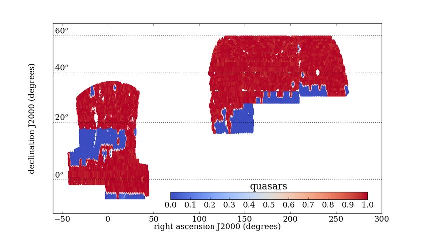
MNRAS 000, 2–19 (2019)                          Preprint 20 July 2020          Compiled using MNRAS LATEX style file v3.0

                                       ABSTRACT
                                       We present the large-scale structure catalogs from the recently completed extended Baryon
                                       Oscillation Spectroscopic Survey (eBOSS). Derived from Sloan Digital Sky Survey (SDSS)
                                       -IV Data Release 16 (DR16), these catalogs provide the data samples, corrected for observa-
                                       tional systematics, and the associated catalogs of random positions sampling the survey selec-
                                       tion function. Combined, they allow large-scale clustering measurements suitable for testing
                                       cosmological models. We describe the methods used to create these catalogs for the eBOSS
                                       DR16 Luminous Red Galaxy (LRG) and Quasar samples. The complementary eBOSS DR16
                                       Emission Line Galaxy catalogues are presented separately in a companion paper, Raichoor et
                                       al. The quasar catalog contains 343,708 redshifts with 0.8 < z < 2.2 over 4,808 deg2 . We
                                       combine 174,816 eBOSS LRG redshifts over 4,242 deg2 in the redshift interval 0.6 < z < 1.0
                                       with SDSS-III BOSS LRGs in the same redshift range to produce a combined sample of
                                       377,458 galaxy redshifts distributed over 9,493 deg2 . The algorithms for estimating redshifts
                                       have improved compared to previous eBOSS results such that 98 per cent of LRG observations
                                       resulted in a successful redshift, with less than one per cent catastrophic failures (∆z > 1000
                                       km s−1 ). For quasars, these rates are 95 and 2 per cent (with ∆z > 3000 km s−1 ). We apply
                                       corrections for trends both resulting from the imaging data used to select the samples for spec-
                                       troscopic follow-up and the spectroscopic observations themselves. For example, the quasar
                                       catalog obtains a χ2 /DoF = 776/10 for a null test against imaging depth before corrections
                                       and a χ2 /DoF = 6/8 after. The catalogs, combined with careful consideration of the details
                                       of their construction found here-in, allow companion papers to present cosmological results
                                       with negligible impact from observational systematic uncertainties.
1   INTRODUCTION                                                          data and random catalogs typically leads to independent public re-
                                                                          leases as SDSS value-added LSS catalog products, with publica-
The Sloan Digital Sky Surveys (SDSS) began in 1998. Since then,           tions describing their creation. For SDSS I and II, the details are in
through phases I and II (York et al. 2000), III (Eisenstein et al.        Blanton et al. (2005)1 . For BOSS in SDSS-III, the details of cat-
2011), and IV (Blanton et al. 2017), they have used the Sloan tele-       alogs extending to z < 0.75 are in Reid et al. (2016). SDSS-IV
scope (Gunn et al. 2006) in order to amass 2.6 million spectra of         eBOSS completed on March 1st, 2019 and obtained four distinct
galaxies and quasars (Ahumada et al. 2019). The primary purpose           samples for studies of large-scale clustering. Here, we describe the
of these observations that simultaneously place a single fiber on         details of the creation of LSS catalogs for eBOSS quasars and lumi-
hundreds of extragalactic objects has been to create three dimen-         nous red galaxies (LRGs). Emission line galaxy (ELG) catalogs are
sional maps of the structure of the Universe. From these maps, we         described in Raichoor et al. (2020) and the Lyman-α forest analysis
observe the large-scale structure (LSS) of the Universe and thereby       of high redshift quasars is described in du Mas des Bourboux, et al.
infer its bulk contents, dynamics, and structure formation history.       (2020).
      During SDSS I and II, the measurement of the location of the             The observed data and random catalogs we produce serve the
baryon acoustic oscillation (BAO) feature in these maps was real-         primary purpose of obtaining BAO and RSD measurements from
ized and developed as a robust and powerful method for obtaining          two-point statistics; i.e., the correlation function in configuration
geometrical measurements of the expansion history of the Universe         space and the power spectrum in Fourier space. The catalogs are,
and thus dark energy (Eisenstein & Hu 1998; Eisenstein et al. 2005;       at their highest level, simply tables with one column for each of
Cole et al. 2005; Percival et al. 2010). This motivated the Baryon        the three dimensions and extra columns that account for selection
Oscillation Spectroscopic Survey (BOSS; Dawson et al. 2013) and           effects or provide weights that optimize these BAO and RSD anal-
extended BOSS (eBOSS; Dawson et al. 2016) programs of SDSS-               yses. The format is meant to allow efficient application of common
III and -IV. During these programs, considerable research was com-        correlation function and power spectrum estimators. While created
pleted in order to use the signature of large-scale redshift-space dis-   to serve this particular purpose, the catalogs are documented and
tortions (RSD; Kaiser et al. 1987) in the maps as a robust measure        made public2 in the hope that they will be useful for any LSS study.
of the rate of structure formation (see Alam et al. 2017 and Alam              For eBOSS, we calculated the catalogs using a development
et al. 2020 for summaries of the developments), thereby allowing          of the MKSAMPLE code, which traces its roots back to BOSS
dynamical tests of dark energy and general relativity.                    Data Release 9 (Anderson et al. 2012), and is described in detail in
      However, in order to confidently use these maps for these           Reid et al. (2016). In essence, MKSAMPLE was a framework for
high-precision cosmological purposes, we must understand and ac-          dealing with the particularities of the SDSS geometry, data model,
count for how the survey design and operation (including all instru-      and observing strategy. Very few of the original lines of code,
mental effects) impact the structure that we record. In essence, at       or even algorithms themselves, are still used in the final eBOSS
every location in the observed space (angles and redshifts), we esti-     MKALLSAMPLES package. However, the underlying philosophy
mate the expected mean density (in the absence of any fluctuations        and basic set of necessary tasks remain almost the same. In this pa-
due to clustering). This is commonly referred to as the survey ‘se-       per, we detail the changes and additions in the eBOSS process and
lection’ or ‘window’ function. It can be Poisson sampled by a set         describe the final catalogs that are produced.
of random positions in the observed space (defined by the survey
design and performance). Variations in the survey selection func-
tion can equally be accounted for by applying weights to either the       1  The updated details for samples through DR7 are available at
data or random catalogs.                                                  http://sdss.physics.nyu.edu/vagc/.
      The complexity (in level of detail) in producing these matched      2 https://data.sdss.org/sas/dr16/eboss/lss/catalogs/DR16/

                                                                                                                            c 2019 The Authors
SDSS DR16 LSS Catalogs 3
This paper is part of a series of papers presenting the com- al. 2000), and III (Eisenstein et al. 2011) surveys using a drift-
pleted eBOSS DR16 dataset and cosmological results derived from scanning mosaic CCD camera (Gunn et al. 1998) on the 2.5-
it, which are summarized in Alam et al. (2020). The DR16 spec- meter Sloan Telescope (Gunn et al. 2006) at the Apache Point
tral reductions described in Ahumada et al. (2019) and the DR16 Observatory in New Mexico, USA. The five-passband (u, g, r, i, z;
quasar catalog produced by Lyke (2020) are vital inputs to the LSS Fukugita et al. 1996; Smith et al. 2002; Doi et al. 2010) photometry
catalogs we create. The LSS catalogs themselves were developed was re-calibrated by Schlafly et al. (2012), who applied the “uber-
in close collaboration with the studies that obtain BAO and RSD calibration” technique presented in Padmanabhan et al. (2008) to
results from the eBOSS DR16 data. For the LRGs, the correla- Pan-STARRS imaging (Kaiser et al. 2010). The photometry with
tion function is presented and used to measure BAO and RSD in updated calibrations was released with SDSS DR13 (Albareti et al.
Bautista et al. (2020), and the power spectrum in Gil-Marı́n et al. 2016) and was demonstrated to have sub-percent level residual cali-
(2020). Rossi et al. (2020) presents the analysis of mock catalogs, bration errors (Finkbeiner et al. 2016). This DR13 photometric data
designed to find and quantify any modeling systematic errors asso- sample was used to inform the optical selection of eBOSS targets.
ciated with the analysis of these data. The equivalent analyses of The infrared data were obtained using the Wide Field Infrared
the quasar sample are presented in Hou et al. (2020), Neveux et Survey Explorer (WISE, Wright et al. 2010). The WISE satellite
al. (2020) and Smith et al. (2020). The ELG catalogs are presented observed the entire sky using four infrared channels centered at 3.4
and analyzed in Raichoor et al. (2020), further analyzed in Tamone µm (W1), 4.6 µm (W2), 12 µm (W3) and 22 µm (W4). We used the
et al. (2020), de Mattia et al. (2020), and supported by simulations W1 and W2 data to identify eBOSS targets. All targeting is based
of the data presented in Alam et al. (2020) and Lin (2020). Multi- on the publicly available unWISE coadded photometry, which ob-
tracer analysis utilizing the overlapping volume between the LRG tained results for SDSS sources via ‘force-matching’ (Lang 2014;
and ELG samples is presented in Wang et al. (2020); Zhao et al. Lang, Hogg & Schlegel 2016)4 .
(2020b). The creation of approximate mocks to be used for covari- The details of the quasar selection are presented in Myers et
ance matrix estimation for all LSS samples is described in Zhao al. (2015), where it was demonstrated that SDSS+WISE imaging
et al. (2020a). Finally the DR16 Lyman-α sample is presented and data can reliably select quasars with 0.9 < z < 2.2. The method
analyzed in du Mas des Bourboux, et al. (2020). A summary of all combined three essential pieces:
SDSS BAO and RSD measurements with accompanying legacy fig-
ures can be found here: https://sdss.org/science/final-bao-and-rsd- (i) XDQSOz (Bovy et al. 2012) reporting a greater than 20 per
measurements/ . The full cosmological interpretation of these mea- cent chance of an object being a quasar at z > 0.9;
surements can be found here: https://sdss.org/science/cosmology- (ii) an extinction corrected flux cut g < 22 or r < 22;
results-from-eboss/ . (iii) a mid-IR-optical color cut, which was proven to be efficient
The types of target (quasar, LRG, ELG) are described in Sec- at removing stellar contaminants.
tion 2, and the targeting criteria for each summarized. In Section 3, An important aspect of the quasar targets is that many were pre-
we describe the eBOSS observing strategy. The method used to viously observed in SDSS I/II/III. Such targets are denoted as
measure redshifts is summarized in Section 4, and the catalog ‘legacy’; the LSS quasar legacy targets were not re-observed.
creation in Section 5. This section also includes details of how we Legacy targets are not isotropically distributed over the sky and
have corrected for many observational effects including varying thus must be treated carefully; these details are provided through-
completeness, collision priority, close pairs, redshift failures, and out Section 5. Ata et al. (2018) demonstrated that selecting quasars
systematic problems with the imaging data. This section ends with that were subsequently measured to have 0.8 < z < 2.2 provided
a review of the statistics for each sample, and provides details of an excellent sample for LSS analyses. Here we will detail how we
how to use these catalogues. A summary of the work is provided have built on these results to provide the final eBOSS quasar LSS
in Section 6. catalogs. The target density is 112 deg−2 within the 6,309 deg2
area planned for eBOSS observation.
The full details of the LRG selection are given in Prakash et
al. (2016). The goal was to obtain a sample at redshifts greater than
the BOSS CMASS sample. In order to make it distinct, the sample
2 EBOSS TARGETS was selected to be fainter in the i-band than BOSS CMASS galax-
eBOSS was designed to acquire redshifts for three types of tracers: ies (Reid et al. 2016). Flux cuts were applied in the i- and z-bands
quasars, LRGs, and ELGs. Each object selected from imaging data in order to obtain targets bright enough to achieve a successful red-
for follow-up spectroscopy is an eBOSS ‘target’. The selection cri- shift. Optical/infrared color cuts achieved a sample with redshifts
teria and motivation for these target samples are detailed elsewhere. mostly greater than z = 0.6, which is near where the density of
Here, we record the essential details. the CMASS ceases to produce cosmic variance limited clustering
measurements. Bautista et al. (2018) demonstrated the sample to
be viable for LSS studies. The target density is 60 deg−2 within the
area planned for eBOSS observation. Here, we provide the details
2.1 Quasars and LRGs on the final LRG sample and combine it with the high redshift tail
LSS quasar3 and LRG targets were selected using the same optical of the BOSS galaxy sample in order to provide one larger sample
and infrared imaging data sets over the full SDSS imaging area. of LRGs with z > 0.6.
The optical data were obtained during the SDSS-I/II (York et Files containing the LRG and quasar target information ap-
3 In order to distinguish this work from the Lyman-α quasar sample, we 4 These data have since been improved as described in Meisner et al.
will denote our sample as ‘LSS quasars’. (2019).
MNRAS 000, 2–19 (2019)4 A. J. Ross et al.
plied to the full SDSS imaging were released5 in DR14 (Abolfathi be placed within 6200 of each other due to the physical size of the
et al. 2018). They can be matched to the ‘full’ files we describe housing of the optical fiber (Dawson et al. 2013). Targets are as-
later (Section 5) using the ‘OBJID TARGETING’ column. signed to ‘collision groups’ via a ‘Friends-of-Friends’ algorithm
with a 6200 linking length (Reid et al. 2016). Any instance where a
target is not observed because it is in a collision group is recorded
2.2 ELGs as a ‘fiber collision’. A fraction of these collisions can be resolved
The eBOSS ELG sample is unique from other eBOSS samples in regions of overlapping plates. The ‘tiling’ algorithm (Blanton
in that it does not use SDSS imaging for its target selection. In- et al. 2003) determines the number of plates and the location of
stead, ELG targets were selected from the DECam Legacy Sur- plate centers in celestial coordinates. In BOSS, tiling over a fixed
vey (DECaLS; Dey et al. 2019) photometric catalog. The details area produced a near-optimal solution of field locations that guar-
of the selection are presented in Raichoor et al. (2017). There, it anteed 100% completeness of non-collided targets for the primary
was demonstrated that within two separate ∼ 600 deg2 regions, a clustering samples. In eBOSS, the 100% completeness requirement
g-band flux cut (g < 22.9(22.825) in the NGC (SGC) region) and was relaxed for the LRG sample to increase the fiber efficiency and
a (g − r)/(r − z) color selection were efficient at producing targets total survey area. In both BOSS and eBOSS, each fixed area that
over the redshift range 0.6 < z < 1.1 with sufficient O[II] flux was tiled in a single software run is referred to as a ‘chunk’. The
to obtain a good redshift. The target catalog was made public6 in eBOSS LRG sample had a completeness of non-collided targets ex-
DR14. Raichoor et al. (2020) present further details on the ELG ceeding 95% in every relevant chunk of the survey. Areas covered
LSS catalog construction and its viability for LSS studies and we by a unique set of plates are ‘sectors’. Completeness statistics are
thus repeat few of them here. determined on a per-sector basis.
LRG and LSS quasar targets were observed on the same
plates, along with targets from the TDSS and SPIDERS programs.
2.3 Other targets TDSS and SPIDERS were each allocated an average surface den-
sity of targets of approximately 10 deg−2 . These plates also con-
Observations of two additional samples of high redshift quasars tained fibers allocated to the two Lyman-α quasar target samples. It
for Lyman-α forest studies (Chabanier et al. 2019; Blomqvist et is possible for any of these samples to overlap in targeting with any
al. 2019; de Sainte Agathe et al. 2019) were also conducted dur- other. Considering one particular sample, e.g., LSS quasars, the fact
ing eBOSS. The first consisted of known z > 2.1 quasars where that it passed another sample’s criteria is generally ignored; i.e., it
increased signal-to-noise would lead to improved cosmology con- is simply treated as any other LSS quasar when constructing the
straints. The second program used multi-epoch imaging data from LSS quasar catalogs. When the target selection criteria are distinct,
the Palomar Transient Factory (PTF; Rau et al. 2009; Law, et al. we must consider the effect of fiber collisions where LRG or quasar
2009) to select high-redshift quasar targets at a density of 20 deg−2 targets could not be allocated fibers because of these additional tar-
in regions with many epochs of photometry (Palanque-Delabrouille gets.
et al. 2016). These provide a random sampling of the foreground
Fiber collisions between different target categories were re-
distribution of neutral hydrogen and do not require a careful record
solved based on the following priority: SPIDERS, TDSS, re-
of the selection function for cosmology studies. The Time Do-
observation of known quasars, LSS quasars, and variability-
main Spectroscopic Survey (TDSS; Morganson et al. 2015) and
selected quasars, with LRGs last. The fiber collision areas occupied
the Spectroscopic Identification of eROSITA Sources (SPIDERS;
by higher priority targets are treated in a ‘veto mask’ that removes
Clerc et al. 2016; Dwelly et al. 2017) programs were also conducted
area from the window function of the desired clustering sample.
simultaneously with eBOSS observations. The Lyman-α, TDSS,
Thus, these priorities result in an LRG sample that covers substan-
and SPIDERS samples do not directly contribute to the clustering
tially less total area than the quasar sample, despite being observed
catalogs presented here, but the footprint of these observations is
at the same time across the same large-scale footprint. See Section
incorporated into the clustering catalogs as will be described be-
5.2 for more details.
low.
A significant portion of the LRG and quasar targets was ob-
served in the Sloan Extended QUasar, ELG and LRG Survey (SE-
QUELS) that was designed as a pilot survey for eBOSS (see Daw-
3 SPECTROSCOPIC OBSERVING son et al. 2016 for details). We treat SEQUELS targets that pass
the eBOSS target selection the same as eBOSS observations, as the
The eBOSS targets were primarily observed using the BOSS
selection is a simple super-set of the ultimate selection. A list of
double-armed spectrographs (Smee et al. 2013) on the 2.5-meter
the chunk numbers is given in Table 1. The SEQUELS targets are
Sloan Telescope (Gunn et al. 2006) at the Apache Point Observa-
covered by chunks boss214 and boss217.
tory in New Mexico, USA. The exception is legacy quasar observa-
ELGs were observed separately from the quasars and LRGs in
tions that used the original Sloan spectrograph. Here, we describe
chunks eboss21, eboss22, eboss23, and eboss25. Some TDSS tar-
the details of the observational strategy and how it impacts our final
gets shared their plates and and were given equal priority. While
sample, while defining key terminology. The details of how spectra
they were observed in separate chunks, the ELG footprint over-
are turned into redshift estimates are presented in Section 4.
laps with the LRG and quasar footprints and thus allows cross-
Like BOSS, eBOSS observed 1000 targets at a time through
correlation studies (e.g., Alam et al. 2019; Wang et al. 2020; Zhao
fibers plugged into holes on pre-drilled aluminum plates. Plates
et al. 2020b).
were placed at the focal plane of the telescope and the fibers fed
directly into the two spectrographs. On each plate, targets cannot Although each chunk was tiled independently, there are some
small regions of overlap in area. In other words, along some chunk
edges, targets were assigned to more than one chunk. To account
5 https://data.sdss.org/sas/dr14/eboss/target/ebosstarget/v0005/ for this duplication, we removed the overlap area from the greater
6 https://data.sdss.org/sas/dr14/eboss/target/elg/decals/ numbered chunk. Doing so provides a unique set of targets over the
MNRAS 000, 2–19 (2019)SDSS DR16 LSS Catalogs 5
Table 1. The eBOSS chunks, the number of tiles in the chunk, and the
number of tiles with good observations in the chunk. (See text for definitions
of ‘chunk’ and ‘tile’; see also Table 1 of Reid et al. 2016.) boss214 and
boss217 were SEQUELS chunks, while chunks 21, 22, 23 & 25 were ELG
plates. All others were standard LRG+QSO plates. SEQUELS tiled further
chunks, which were unobserved at the end of the survey: the area in these
chunks was recovered by eBOSS chunks, but without any overlap in the
tiles.
chunk # of tiles # of good tiles
boss214 148 88
boss217 74 29
eboss1 199 195
eboss16 128 127
eboss2 98 81
eboss20 42 42
eboss21 46 46
eboss22 121 121
eboss23 87 85
eboss24 81 51
Figure 1. The footprint of eBOSS targets. Black points show LRG and
eboss25 51 51
quasar targets that were tiled but did not obtain spectroscopic observations
eboss26 171 76
(see text). Yellow points show quasars that were observed. They almost
eboss27 94 37
entirely overlap the red points, which show LRGs that were observed. Blue
eboss3 204 180
points show 20 per cent of the ELGs that were observed. The gray points
eboss4 80 80
are BOSS CMASS galaxies from their LSS catalogs. The CMASS data has
eboss5 70 70
their veto masks applied, while no such masks are applied for the eBOSS
eboss9 34 34
data in this plot. The eBOSS LRG and quasar footprints with veto masks
applied are shown in Section 5.4 and the equivalent ELG footprint is shown
in Raichoor et al. (2020).
points, which show the quasars that were observed. One can ob-
full eBOSS footprint. However, we always take the highest quality serve an area at ra, dec ∼ 225, 55 where there are no quasars. In
spectrum for duplicate tilings of the same target. For example, if this area, SDSS had previously obtained spectra for all of the quasar
a target received a fiber in both chunks eboss20 and eboss26 and targets (incorporated into the special Reverberation Mapping pro-
the better spectrum was observed in eboss26, the redshift from the gram; Shen et al. 2015) and thus eBOSS did not re-observe them.
eboss26 observation is assigned. However, if the target in eboss20 The blue points display twenty per cent of the ELGs that were ob-
was not assigned a fiber (e.g., due to a collision), but gets observed served. This subsampling allows one to see the overlap with the
in eboss26, the eboss26 observation is not used in the clustering cat- LRG and quasar samples. The overlap of the ELG sample is com-
alogs. This avoids biasing the selection probabilities within these plete in the South Galactic Cap (SGC; the filled area in the figure
regions. Such cases are fairly rare and are treated as if no fiber was with right ascension < 60). In the North GC (NGC), the ELG data
placed on the target. The geometry file described in Section 5 cuts fully overlaps with the BOSS CMASS data, but the eBOSS LRG
between chunks at the boundary of the highest-numbered chunk, and quasar footprint only covers approximate half of the NGC ELG
corresponding to this selection. footprint.
In many cases, eBOSS chunks that were tiled did not have all
of their plates observed. This is the primary source of incomplete-
ness in the eBOSS catalogs. We denote the following classifica-
4 DETERMINING REDSHIFTS
tions that lead to incompleteness for an eBOSS target within a tiled
chunk: The IDLSPEC 2 D spectral reduction pipeline reduces every eBOSS
• ‘close-pair’: No fiber was placed on the target due to a fiber colli- spectrum from a series of two-dimensional images that span multi-
sion (un-resolved with overlapping plates) with a target of the same ple exposures, to a single, wavelength-calibrated, one-dimensional
class. spectrum. The spectra that were used to generate the catalogs pre-
• ‘missed’: No fiber was placed on the target, not due to it being sented in this paper were processed with version V 5 13 0 of the
a close-pair. Observations will be missed primarily due to missing data reduction pipeline. This is the final version of the IDLSPEC 2 D
plates in overlap regions and can also occur when more than 1000 software that will be used to process clustering data obtained with
fibers would have been required to observe all targets in a given the SDSS telescope. A summary of the improvements to this soft-
region. ware package over the course of eBOSS can be found in the studies
• ‘wrong-chunk’: A fiber was placed on the target only in the that first incorporated those improvements (Hutchinson et al. 2016;
greater-numbered overlapping chunk. Jensen et al. 2016; Bautista et al. 2017) and in the DR16 paper
Fig. 1 displays the sky positions of eBOSS targets that were (Ahumada et al. 2019).
tiled. The black points are LRG and quasar targets that were not As in SDSS and BOSS, every spectrum is then assigned a clas-
observed. The colored points display eBOSS targets observed with sification of star, galaxy, or quasar, a redshift, and a quality flag
plates determined to be ‘good’. The red points are LRG targets that indicates the robustness of the redshift estimate. The redshift
that were observed. They are mostly overlapped by the yellow catalogs associated with DR16 exactly follow the procedures de-
MNRAS 000, 2–19 (2019)6 A. J. Ross et al.
scribed in Albareti et al. (2016) and Bolton et al. (2012). However, The redshift and spectral class that give the lowest value of χ2 are
different philosophies for redshift estimates and spectral classifica- considered the best description of the spectrum. A fit is only con-
tion were designed specifically for the eBOSS LSS catalogs. A new sidered reliable, or good, if it can be differentiated from the second
redshift estimate pipeline for galaxies was motivated by the chal- best fit by a sufficiently large difference in the χ2 . We denote this
lenges faced with the low signal-to-noise galaxy spectra. A new parameter as ∆χ2 .
scheme that supplemented automated classifications with visual in- The first improvement over the BOSS fitting routines was the
spections was developed to characterize the very large number of introduction of the instrument resolution to the spectral models.
quasar spectra obtained in eBOSS. We describe the new algorithms Each model is generated at a significantly higher resolution than
customized to LRG spectra in Section 4.1 and briefly summarize offered by the BOSS spectrograph. At each redshift, the model is
the procedures for ELG and quasar spectra in Section 4.2 (these are convolved with the wavelength-dependent estimate of the Gaussian
described in greater detail in Raichoor et al. 2020; Lyke 2020). profile that describes the instrument resolution for that spectrum.
The relative success of classification is divided into three The inclusion of instrument performance in this step allows better
cases: good redshift, redshift failure, and no chance of good redshift characterization of narrow spectral lines, particularly when there is
(‘bad fiber’). For all three LSS tracers, the bad fibers are determined a strong variation in the resolution as a function of wavelength as
based on the ZWARNING flag from the eBOSS pipeline. Observa- often occurs near the detector edges.
tions with bits 1 (‘LITTLE COVERAGE’), 7 (‘UNPLUGGED’), 8 The second improvement over the BOSS fitting routines is
(‘BAD TARGET’), or 9 (‘NO DATA’) had no chance of obtaining an introduction of new spectral templates for galaxies and stars9 .
a good redshift and are classified as bad fibers. As the cases of bad Galaxy spectral templates are derived from a principal component
fibers are uncorrelated with the target properties, they are treated analysis (PCA) decomposition applied to a total of 20,000 theoret-
in the same manner as if they did not receive a fiber in the catalog ical galaxy spectra (Charlie Conroy 2014, private communication)
creation, as described in Section 5.4. The following subsections de- that span stellar age, metallicity, and star formation rate10 . Emis-
tail how we classify between good redshifts and failures for LRGs sion lines of varying equivalent width were painted onto the the-
and quasars. We describe the characterization of the spatial varia- oretical galaxy spectra. The resulting PCA eigenspectra are there-
tion of redshift failures and our statistical corrections for them in fore physically-motivated, as opposed to the BOSS eigenspectra
Section 5.3. that were derived empirically from early data and are thus degraded
from noise and occasional spurious signal in the spectra. There are
10 galaxy PCA eigenspectra templates that are used in linear com-
4.1 Redrock Redshift Estimates for the LRG Sample bination to obtain redshifts for the entire eBOSS galaxy sample.
The stellar templates were also derived from a series of the-
As discussed in Dawson et al. (2016), the spectra from the BOSS
oretical models divided approximately by stellar mass and evolu-
CMASS galaxy sample had sufficient signal-to-noise to enable
tionary stage. The stellar templates were motivated by laboratory
very reliable automated redshift classification using the same al-
atomic data, molecular data, and model atmospheres (Allende Pri-
gorithms as those in the recently released DR16 catalogs. How-
eto et al. 2018, Allende-Prieto et al. private communication). A to-
ever, early in SDSS-IV, it became clear that these routines are not
tal of 30,000 template stars were used. 10,000 had spectral types
optimized for the fainter, higher redshift LRG galaxies that com-
A, B, F, G, K, or M. 20,000 white dwarf templates were used, split
prise the eBOSS LRG sample. When first applied to the eBOSS
evenly between types DA and DB. Broad TiO absorption features
samples, only about 70% of the spectra were given good redshifts.
in red dwarf spectra can masquerade as G-band or balmer breaks in
The high rate of redshift failures motivated the new development in
high redshift galaxies. Thus, extra care was taken to increase the di-
the IDLSPEC 2 D spectral reduction pipeline for higher quality one-
versity of M-type and K-type main-sequence stellar templates. The
dimensional spectra. More significant improvements to the rate of
introduction of these new templates was proven to reduce the rate of
good redshift estimation were achieved through a new approach to
false detections around z = 0.62 and z = 1.02. The CV-type stel-
redshift estimation.
lar templates and the four quasar eigenspectra produced by Bolton
The new redshift algorithm, REDROCK7 , was developed for
et al. (2012) and used in previous eBOSS analyses were copied
the Dark Energy Spectroscopic Instrument (DESI; Aghamousa et
into REDROCK. The redshifts for the LSS quasar sample were de-
al. 2016a). The REDROCK team used an improved combination of
termined determined as detailed in the following subsection (not by
the Bolton et al. (2012) approach and an archetype (Cool et al.
REDROCK ).
2013) approach similar to that applied in REDMONSTER (Hutchin-
In the second element of the REDROCK redshift classification
son et al. 2016). Methods developed in Zhu (2016)8 were incorpo-
scheme, a subset of the spectral templates described above were
rated in order to provide additional improvements. We describe the
used as archetype models11 to fit the spectra in a manner similar
approach in more detail throughout the rest of this section.
to REDMONSTER. The motivation for this second step was to apply
The general process, which we expand on below, is as follows:
an additional filter on the spectral fitting and exclude non-physical
Classification and redshift determination are performed via a fit of
combinations of the eigenspectra that can generate erroneous red-
a linear combination of spectral templates to each spectrum. Fitting
shift detections. Archetype fitting was not performed over the full
is done over a range of redshifts for three different classes of tem-
redshift range, but instead was performed only over the range of
plates that independently characterize stellar, galaxy, and quasar
within 10,000 km s−1 of the redshift estimate from a maximum
spectral diversity. Unlike the approach used in the BOSS redshift
of the three best-fit cases for each class (galaxy, quasar, star) from
pipeline, no nuisance terms are allowed to soak up flux calibration
errors, intrinsic dust extinction, or other sources of spurious signal.
9 https://github.com/desihub/redrock-templates; tagged version 2.6
10 Specifically, these are broken up by DESI target class to have 10,000
7 https://github.com/desihub/redrock; tagged version 0.14.0 ELGs, 5,000 LRGs, and 5,000 spectra representing the flux-limited ‘Bright
8 Parts of this associated code were used: Galaxy Sample’
https://github.com/guangtunbenzhu/SetCoverPy. 11 https://github.com/desihub/redrock-archetypes; tagged version 0.1
MNRAS 000, 2–19 (2019)SDSS DR16 LSS Catalogs 7
the first stage of classification. For the redshift ranges where the dicates a systematic bias in the algorithm in the limit approach-
spectral class was estimated to be a galaxy, 110 archetype galaxy ing zero signal. We have not been able to identify the source of
templates were fit in combination with nuisance terms that con- this bias. The spectra failing to meet the physicality condition are
trol the amplitude of the first three Legendre polynomials, meant shown in red in Figure 2. One notes that these pairs are most likely
to fit non-physical flux in the broadband spectrum. Likewise, 40 found at low values of ∆χ2 , as would be expected. There are only
stellar archetype spectra were fit to the spectrum for the redshifts 0.04 per cent of LRG spectra in the full eBOSS sample that satisfy
where the PCA spectral class was estimated to be stellar, and 64 the ∆χ2 = 9 condition but fail to meet this threshold on posi-
archetypes were fit for class quasar. The redshift and class that pro- tive archetype coefficients. Given the results on the sky spectra, we
duced the lowest value of χ2 was then considered the best descrip- can expect a similar percentage of catastrophic failures in our LRG
tion of the spectrum. The results from the archetype fits superseded sample due to these false-positive confident redshifts; i.e., this is a
those from the PCA eigenspectra fitting and are used for the clus- negligibly small fraction. The requirement that the first coefficient
tering catalogs. The ∆χ2 between the best two archetype fits was be positive for the best-fitting archetype spectrum removes spuri-
recorded and later used to define our redshift failure criteria. ous detections from non-physical fits to the data, albeit at a very
To limit the number of interlopers in our LSS measurements, low rate.
we established a requirement that limited the number of misclassi- After final classifications, the redshift completeness now ap-
fied, or ‘catastrophic failures’, to be less than 1%. A catastrophic proaches 98% for the eBOSS LRG sample with a rate of catas-
failure for galaxies occurs when an object is confidently assigned a trophic failures estimated to be less than 1%. These cases of catas-
redshift that is in error by more than 1000 km s−1 . The final tuning trophic failures appear in the clustering catalogs without correction
to discriminate between good redshifts and redshift failures and to but are shown to be sufficiently rare as to not bias the cosmological
assess the resulting rate of catastrophic failures was done empiri- measurements. Stars are a major contaminant, as they make up 9%
cally using multi-epoch spectra and sky spectra, as described below. of the spectral classifications for the LRG sample. An additional
We use a sample of multi-epoch spectra to identify a value of one per cent of spectra are classified as quasars and not used in the
the ∆χ2 that maximizes the number of good redshifts while main- LSS catalogs. In total, 88 per cent of LRG observations result in a
taining sufficient purity in the catalog. Many of these objects re- good LRG redshift.
ceived more than one observation due to intentional reobservations
of a plate while others had multiple fiber assignments in the regions
of plate overlap. There were 11,556 pairs of spectra used to perform 4.2 ELG and Quasar Redshift Estimates
this test. For each pair of spectra, we determined the difference in
We also utilize the REDROCK code to make redshift estimates for
the redshift estimates, ∆v. The distribution of ∆v is shown in the
the ELG spectroscopic sample. The PCA and the archetype spec-
left panel of Fig. 2 while the results as a function of ∆χ2 are pre-
tral templates are identical to those described above. The require-
sented in the right panel. Using the fit to the distribution, which we
ment for ∆χ2 between models and the restriction on the archetype
have cut to the 0.6 < z < 1.0 redshift range used for the clustering
coefficients are also identical. However, two additional criteria are
catalogs, the√mean redshift uncertainty for the LRG sample is 65.6
applied to the ELG program: the median signal-to-noise per pixel
km s−1 (1/ 2 the width of the distribution in Fig. 2). An uncer-
must exceed 0.5 in either the i−band or z−band region of the spec-
tainty of this scale is small compared to typical peculiar velocities
trum and the measured continuum or [OII] emission line strength
and is thus absorbed into their modeling in the LSS analyses.
must also pass the a posteriori flags defined and motivated in Com-
We then assessed the rate of catastrophic redshift failures by
parat et al. (2016) and Raichoor et al. (2017); the criteria using these
counting the fraction of pairs that produced redshift estimates dif-
flags is (zQ >= 1 or zCont >= 2.5). The details of purity and
fering by more than 1000 km s−1 . For a threshold ∆χ2 = 9 (re-
completeness after each of these filters is presented in Raichoor et
jecting 761 pairs), we find that 0.5% of the 10,795 pairs produced a
al. (2020). We are able to obtain secure redshifts for 91% of ELG
catastrophic redshift failure. Under the assumption that one of the
observations with a catastrophic failure rate of less than 1%.
redshift estimates in the pair was correct, the resulting catastrophic
We use a multi-stage process to determine the redshift and
failure rate is estimated to be 0.25%.
quality indicator for the quasar sample. This process follows on
We then applied an additional level of filtering to further re-
the philosophy of Pâris et al. (2018) and is fully described in Lyke
duce the rate of catastrophic failures, which was to require a posi-
(2020), which presents the ‘DR16Q’ quasar catalog. From these
tive amplitude for the coefficient of the best-fitting archetype spec-
results, we used the following criteria to determine redshift fail-
trum. In cases where the best fitting redshift was produced by an
ures: if an object was not classified as a quasar by the automated
archetype template with a negative amplitude, we kept that red-
decision-tree described in Lyke (2020)13 and had an IDLSPEC 2 D
shift but set a flag indicating that the redshift was not to be trusted.
ZWARNING flag set (not associated with the bad fibers described
These are counted as redshift failures in the down-stream analysis.
above), it was typed as a redshift failure. If no ZWARNING flag
We applied this condition based on tests of 365,243 sky-subtracted
was set, the observation was assigned the classification determined
sky spectra. Without the requirement, we found that 10 per cent of
by the IDLSPEC 2 D pipeline. Additionally, anything with a median
these sky spectra were given a confident redshift estimate12 using
signal-to-noise < 0.5 per pixel across the spectrum was classi-
the ∆χ2 = 9 threshold, whereas one would expect a negligible
fied as a redshift failure. All redshifts we use in the LSS cata-
fraction of astrophysical spectra in those fibers. With the require-
logs were determined using the REDVSBLUE14 principle compo-
ment, this was reduced to 4.4 per cent. While the positive-archetype
nent analysis (PCA) algorithm described in Lyke (2020) and stored
requirement provides a significant improvement, this behavior in-
in the Z PCA column within DR16Q. Within our redshift range of
12 These ‘redshifts’ broadly sample the allowed redshift range with only 13 This classification is stored in the column named ‘MY CLASS PQN’
minor structure that appears to be caused by confusion from sky subtraction in the ‘full’ quasar catalog files.
artifacts. 14 https://github.com/londumas/redvsblue
MNRAS 000, 2–19 (2019)8 A. J. Ross et al.
eBOSS LRG repeats - redrock 11556 pairs
eBOSS LRG - 8072 pairs with ∆χ2 > 9.0 106
Gaussian fit µ = 1.3, σ = 91.8 105
0.005
104
Normalized distribution
0.004
103
∆v (km/s)
0.003 102
101
0.002
100
0.001
10−1
0.000 10−2
−400 −200 0 200 400 10−1 100 101 102 103 104
∆v (km/s) 2
∆χ
Figure 2. Left: The distribution of ∆v over 8,071 pairs of observations of the same LRG target at 0.6 < z < 1.0 and with confident detections (∆χ2 > 9).
∆v is the difference in velocity between two redshift measurements of the same object. The solid line shows the best-fit Gaussian model to the distribution
after requiring |∆v| < 250 km s−1 . The mean and dispersion are shown in the legend. Right: ∆v as a function of ∆χ2 , for 11,556 pairs where we apply no
cut on redshift. ∆χ2 represents the statistical difference between the best and the second best fit spectral template to a single spectrum. The lower ∆χ2 in the
pair is considered the independent parameter. Pairs in which one spectrum was fit with an archetype spectral template with negative amplitude are presented
in red. The horizontal red dashed line shows the limit of ∆v = 1000 km/s above which a pair is considered as a catastrophic failure. The dotted vertical line
shows the ∆χ2 = 9, below which results are classified as redshift failures.
0.8 < z < 2.2, we find this redshift performs well both in terms ∆v > 3000km s−1 relative to the REDVSBLUE redshift. These
of systematic and statistical uncertainties, as discussed below.15 Vi- combine for an estimated 2 per cent catastrophic failure rate on
sual inspection information is only used to evaluate the catastrophic LSS quasar targets observed by eBOSS. All legacy redshifts had
failure rate, as described below. been visually inspected prior to eBOSS and determined to be good
The process results in 95 per cent of quasar target observa- quasar redshifts. Legacy quasars make up 18 per cent of the quasar
tions having a good redshift with a quasar, stellar, or galaxy clas- redshifts used in the LSS catalogs with 0.8 < z < 2.2. We thus
sification. Seven per cent of the observations are typed as galaxies estimate the total catastrophic failure rate to be 1.6 per cent for the
and two per cent stars. In total, 86 per cent of the eBOSS quasar LSS quasar sample (as the total fraction is 0.02×0.82).
observations are classified as having a good quasar redshift. This statistical characterization of the distribution of redshift
The statistical uncertainties in quasar redshift estimates are on uncertainties in our LSS quasar catalog is used in Smith et al.
computed empirically using repeat observations. Lyke (2020) find (2020) to create simulations that are consistent with these results.
a typical statistical redshift error of 300 km s−1 without strong red- Thus, Hou et al. (2020); Neveux et al. (2020) are able to deter-
shift dependence. Systematic errors in redshift estimates are some- mine the sensitivity of their BAO and RSD measurements to such
what more difficult to assess, as the emission lines that inform the redshift uncertainties and catastrophic failures and incorporate the
fits are subject to internal dynamics and can be shifted with respect results into their systematic error budgets.
to the quasar rest-frame. Lyke (2020) study this by using results
of repeat observations from the Reverberation Mapping program
(Shen et al. 2015) and find no evidence of a systematic uncertainty 4.3 Redshift Distributions
in the PCA redshifts with the range 0.8 < z < 2.2; see their figure
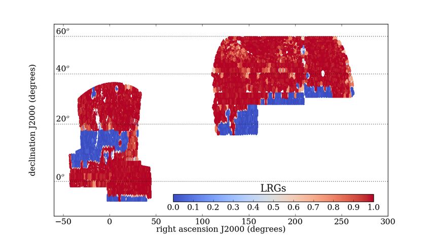
Figure 3 displays redshifts from the samples used to create eBOSS
3.
LSS catalogs. The SDSS I/II/III quasars were selected as eBOSS
Catastrophic failures are characterized via the 10,000 ran-
LSS quasar targets. These already had secure redshifts determined
dom visual inspections described in Lyke (2020). From this set
by visual inspection. Thus, for the LSS quasar sample, we use their
of 10,000, we select the LSS quasar targets that were classified as
previously observed spectra and redshift estimates rather than re-
quasars and had eBOSS (not legacy) redshifts 0.8 < z < 2.2.
observe them. See Section 2 for more details. These legacy quasars
This sample provides a base set of 5,449 objects that we include
span the whole redshift range and comprise approximately one
as good quasar redshifts in our clustering catalogs. Of these, the
quarter of the total quasar redshifts. The BOSS galaxies were not
visual inspection found 1.2 per cent (63) were not quasars16 . An
targeted by eBOSS, but we will use BOSS CMASS galaxies at
additional 0.8 per cent (45) were determined to have redshifts with
z > 0.6 in order to create one combined sample of luminous galax-
ies with z > 0.6.
15 For the Lyman-α forest studies presented in du Mas des Bourboux, et
al. (2020) Z LYAWG is used instead, where Lyman-α emission is masked.
This is less of a concern in our redshift range. 5 CATALOG CREATION
16 No accurate new classification or redshift estimate was attempted but
any resulting redshift would have been unlikely to be close to the original In this section, we detail the catalog creation steps for the LRG and
‘quasar’ redshift’ quasar samples. The steps are similar for the ELGs, but those cata-
MNRAS 000, 2–19 (2019)SDSS DR16 LSS Catalogs 9
photometry18 and the columns ‘PLATE’, ‘MJD’, ‘FIBERID’ to
match to the publicly available spectra19 .
• A table with rows for only the data with good redshifts, with
all mask, completeness, and redshift cuts applied. It contains only
the columns that are necessary for calculating two-point statistics
and matching to the full file. We denote these the ‘clustering’ files.
• A table of random points approximating the selection function
of the clustering file for the data, to be processed in the same way
as the data file for the calculation of two-point statistics.
The clustering files are produced separately for each Galactic hemi-
sphere.
5.1 Matching Targets and Spectroscopic observations
The galaxy catalog creation starts from the target sample. The infor-
mation for all eBOSS targets within tiled chunks is collated. From
this master list of eBOSS targets, the target sample in question is se-
lected. Each target sample is then matched to spectroscopic obser-
Figure 3. Histograms of the redshifts of samples used in eBOSS LSS anal- vations. A first step is to cut the spectroscopic information to unique
yses. The quasars are selected to pass our LSS sample target selection, as
entries per target. For LRGs, this is done by selecting primary spec-
explained in the text, but many were already observed by previous gener-
troscopic observations from the SDSS database (SPECPRIMARY
ations of SDSS. The SDSS-III BOSS CMASS sample is included, as we
combine this sample with eBOSS LRGs to produce one larger sample. = 1). For quasars, we use the DR16Q superset (Lyke 2020) catalog
as the source of redshifts. The primary record (PRIM REC =1) is
selected.
logs are described in Raichoor et al. (2020). The order for catalog For the quasars, we first match the legacy targets with their
creation is: spectroscopic information. These objects were flagged in the target
file as having already been observed and thus were removed from
• create randoms at constant surface density within the tiled consideration by the tiling algorithm. We match these targets to
footprint; DR16Q, populate the relevant spectral information (redshift, object
• match between targets and spectroscopic observations; type, etc.), and denote them as legacy. We then match the remaining
• apply veto masks; targets based on their internal ID. For the LRGs, we go straight to
• resolve fiber collisions and determine completeness; matching based on internal ID.
• assign weights to correct for fiber collisions and redshift fail- After this matching, the following classifications are possible,
ures; which are stored as an integer value in the ‘IMATCH’ column of
• cut on redshift and completeness; the ‘full’ file:
• assign weights that correct for systematic trends with fore-
grounds and imaging meta data; • a target can remain unobserved (IMATCH=0); denoted missed ,
• assign redshift related information to random catalogs. • have a good eBOSS redshift that matches the targeted type
(IMATCH=1; denoted z,eboss ),
Many of these steps apply to both the data catalog and the ran- • have previously been determined to be a quasar with a good
dom catalog that is used to quantify the window function. The first legacy redshift (IMATCH=2; denoted leg , relevant only for quasar
operation is therefore to create a catalog with random angular posi- targets),
tions at a density of 5000 deg−2 within the geometry of the full tiled • be a star (IMATCH=4; denoted star ),
area, which is more than 40 times greater than the target density of • be a redshift failure (IMATCH=7; denoted zfail , see Section
the quasar sample (and more than 70 times greater than the LRG 4),
target density). This area is a collation of the previously described • be identified as an object of the wrong target type (e.g., an
chunks (with overlap removed) and occupies 6309 deg2 . A polygon LRG target is identified to be a quasar; IMATCH=9; denoted
file that can be used with M ANGLE (Swanson et al. 2008) named badclass ),
‘eBOSS QSOandLRG fullfootprintgeometry noveto.ply’ • have previously been determined to be a legacy star
defines this geometry, with a corresponding FITS17 file that allows (IMATCH=13; relevant only for quasar targets),
a mapping between polygons and sectors. • be a bad fiber (IMATCH=14, see Section 4),
For each tracer, we release files containing the following types • or was not tiled in its target chunk (IMATCH=15, see Section
of tables: 3).
• A table with a row for every unique target that was tiled and Objects with IMATCH=14,15 are treated the same as unobserved
passes the veto masks; we denote these the ‘full’ files. They con- objects for calculating all subsequent statistics, i.e., we tabulate
tain all of the information on the target’s photometry and spec- any quantity with the subscript missed including the IMATCH=14
tra (if observed) and relevant IDs. One can use the column ‘OB- and 15 objects. Some IMATCH=2 objects will get re-assigned as
JID TARGETING’ to match to ‘objID’ in the publicly available
18 https://www.sdss.org/dr16/imaging/
17 https://fits.gsfc.nasa.gov/fits standard.html 19 https://www.sdss.org/dr16/spectro/spectro access/
MNRAS 000, 2–19 (2019)10 A. J. Ross et al.
IMATCH=8, based on completeness considerations, as described ples were observed on different plates and in different chunks, so
in Section 5.4. IMATCH 5 and 6 are not used. the observation of one has no impact on the other.
In general, the veto masks were not applied to the target sam-
ples. Thus, many good redshifts were observed within these vetoed
5.2 Veto Masks regions. For example, for the Bright Star and Bad Field masks, we
do not trust that the photometry used to produce the target samples
After the matching and type assignment, a series of veto masks are should produce isotropic samples suitable for large-scale structure.
applied to the targets and randoms. These masks and statistics de- These areas thus tend to have proportionally fewer good redshifts.
scribing what they remove are detailed in Table 2. Chunks covering Across all veto masks, for LRGs, nine per cent of the good redshifts
a unique area of 6309 deg2 were tiled for observation. Approxi- are vetoed, to be compared to 17 per cent of the tiled area. For the
mately 500 deg2 of the area is vetoed from the quasar footprint quasars, we lose 4.5 per cent of the good redshifts while removing
and more than 1000 deg2 is vetoed from the LRG footprint. Four 7.1 per cent of the tiled area.
veto masks are applied to each of the LRG and quasars. The bad
field, bright star, and bright object masks are the same as applied to
BOSS DR12 (Reid et al. 2016). The centerpost mask removes the 5.3 Spectroscopic Completeness Weights
area at the center of the plate where no target can be observed (the
After the veto masks were applied, ‘close pairs’, denoted cp ,
centerpost pulls the center of the plate such that its curvature ap-
were assigned. Any object without a spectroscopic observation that
proximately matches the best-focus surface, see Smee et al. 2013).
shares a collision group with an object that obtained a spectroscopic
The infrared bright star mask was applied to the LRG sample,
observation is typed as a close pair and given IMATCH = 3. The
as it was found that many spurious LRG targets exist around these
distributions of these close pairs and also the redshift failures are
stars. The size of the region that was masked is based on the WISE
not expected to be isotropic and close pairs are expected to be cor-
W 1 magnitude, unless the 2MASS K-band magnitude was less
related with the density field itself. These sources of spectroscopic
than 2. Around each source, a circular region of 55000 was removed
incompleteness require special treatment.
from consideration if either W 1 or K was less than 2 magnitudes.
For the close pairs, the weights are assigned and equally dis-
For fainter sources up to W 1 = 8 we applied
tributed per collision group. All good observations in a collision
rIRmask = (1397.5−569.34W 1+79.88W 12 −3.75W 13 )00 . (1) group receive a weight that is
Ncp + Nz,eboss + Nbadclass + Nstar
Based on early data occupying 800 deg2 , 85 per cent of LRG targets wcp = , (2)
Nz,eboss + Nbadclass + Nstar
removed by this mask were not LRGs. Thus, the mask was applied
to LRG targets used for tiles eboss9 and greater so that the fibers where the N are summed within each of these groups. Such a
could be assigned to targets more likely to produce good redshifts. weighting provides unbiased transverse clustering on large-scales
These IR stars were not found to have any impact on quasar targets, in configuration space. However, the radial clustering will be bi-
beyond what is masked by the regular bright star mask. ased, and the issues are more severe in Fourier space (Hahn, et al.
The collision priority mask removes the 6200 radius area 2017). Bianchi & Percival (2017) provide an unbiased solution for
around where higher priority targets prevent any fiber to be as- configuration space and Mohammad et al. (2020) presents an ap-
signed to the given target type. The LRGs had the lowest prior- plication of these weights to eBOSS data. However, in the standard
ity and the area of collision priority mask applied for them is thus catalogs we simply provide wcp and each individual analysis de-
nearly 700 deg2 . The overlapping plate geometry allows collisions scribes how the size of any remaining systematic biases how they
between lower-priority LRGs and higher-priority targets to be re- are treated.
solved. However, these collisions are not fully resolved and some We provide corrections for redshift failures based on the spec-
LRGs remain unobserved in these regions. We thus apply the con- trograph signal-to-noise in the i-band and the fiber ID. The like-
servative option of masking 6200 around every higher-priority target lihood of obtaining a good redshift naturally correlates with the
and accept losing the 10,439 good redshifts in this mask. signal-to-noise of the spectrum. The fiber ID correlates with the
Only TDSS and SPIDERS have greater priority than the location of the spectrum on the CCD of the spectrograph, which
quasars. Also, the quasar collisions in regions with overlapping in turn alters the signal-to-noise of the spectrum. The fiber ID also
plates are fully resolved. Thus, we only apply the quasar collision correlates with the expected location on the plate, resulting in large-
priority mask in single tile regions. This mask is only 66 deg2 for scale signal-to-noise variations across the sky.
the quasars and only 39 of the more than 7000 quasar targets re- We fit for trends between these quantities and the redshift ef-
moved by this mask have good redshifts; the number is greater than ficiency, as defined below, and use the inverse of the trends as a
0 only due to the fact that the center of the veto regions are within weight. We define the number of good spectra associated with a
the single tile region but can extend out into the area with overlap- particular data subsample20 as
ping tiles.
Ngoodz = Nz,eboss + Nbadclass + Nstar . (3)
Note that by applying the veto masks to both galaxies and ran-
doms, we are implicitly assuming that the regions removed are un- NalleBOSS is then Ngoodz + Nzfail and the redshift efficiency for
correlated with the cosmological density fluctuations that we want any particular sub-sample is thus
to measure. This may be a slight concern where higher-priority tar-
Ngoodz
gets overlap in redshift with the sample of interest. The main con- fgood = . (4)
NalleBOSS
cern is clustering between z < 1 quasars and our LRG sample. We
apply no correction for this and expect it to be a minor effect on
the LRG clustering given the substantially lower projected number 20 A subsample can be, e.g., all spectra associated with a spectrograph on
densities of z < 1 quasars compared to 0.6 < z < 1 LRGs. This is a single plate, all of the spectra associated with a given fiberID over all
not an issue for the ELG/LRG multi-tracer analysis, as these sam- eBOSS observations, etc.
MNRAS 000, 2–19 (2019)You can also read