The economic contribution of Melbourne's foodbowl - A report for the Foodprint Melbourne project, University of Melbourne - Deloitte
←
→
Page content transcription
If your browser does not render page correctly, please read the page content below
The economic
contribution of
Melbourne’s foodbowl

A report for the Foodprint
Melbourne project, University
of Melbourne
July 2016
Contents
Key points ........................................................................................................................ i
Executive Summary ......................................................................................................... ii
1        Introduction .......................................................................................................... 1
2        Profile of Melbourne’s foodbowl ........................................................................... 2
         2.1       Melbourne’s foodbowl........................................................................................... 2
         2.2       Agricultural production in the foodbowl ................................................................. 3
         2.3       Food manufacturing activities ................................................................................ 6
         2.4       Food consumption in Melbourne ........................................................................... 7
3        Economic contribution of Melbourne’s foodbowl ................................................ 12
         3.1       Methodology ....................................................................................................... 12
         3.2       Results................................................................................................................. 13
4        Economic impacts under alternative future scenarios.......................................... 15
         4.1       Methodology ....................................................................................................... 15
         4.2       Melbourne growing to accommodate 7 million people......................................... 16
         4.3       Increasing preference for ‘local’ food ................................................................... 21
5        Ancillary benefits................................................................................................. 24
         5.1       Insurance and option value .................................................................................. 24
         5.2       Visual amenity ..................................................................................................... 25
         5.3       Other ancillary benefits........................................................................................ 26
         5.4       Future ancillary benefits ...................................................................................... 27
         5.5       Note on ancillary benefits .................................................................................... 28
6        Conclusion .......................................................................................................... 29
Appendix A Input-Output analysis ................................................................................. 31
Appendix B CGE modelling ............................................................................................ 33
Appendix C Local Sourcing assumptions ........................................................................ 37
         References ..................................................................................................................... 38
         Limitation of our work .................................................................................................... 41

Charts
Chart 2.1 Victorian agricultural land, by region ................................................................ 4
Chart 2.2 Value of Agricultural Production in Melbourne’s foodbowl, by LGA .................. 4

Liability limited by a scheme approved under Professional Standards Legislation.

Deloitte refers to one or more of Deloitte Touche Tohmatsu Limited, a UK private company limited by guarantee, and its
network of member firms, each of which is a legally separate and independent entity.
Please see www.deloitte.com/au/about for a detailed description of the legal structure of Deloitte Touche Tohmatsu Limited
and its member firms.

© 2016 Deloitte Access Economics Pty Ltd
Chart 2.3 Gross value of agricultural production in Melbourne’s foodbowl...................... 5 Chart 2.4 Persons employed in agriculture in the foodbowl, food production only .......... 6 Chart 2.5 Employment in selected food processing industries, by region ......................... 6 Chart 2.6 Average daily dietary intake, by food category ................................................. 8 Chart 2.7 Population of Greater Melbourne, 2011 to 2051 .............................................. 9 Chart 2.8 Melbourne’s food demand now and in future (thousand tonnes) ................... 10 Tables Table 2.1 : Definition of foodbowl areas .......................................................................... 2 Table 3.1 Economic contribution of agriculture and food manufacturing in Melbourne’s foodbowl ...................................................................................................................... 13 Table 3.2 Sectoral economic contribution in Melbourne’s foodbowl ............................. 14 Table 4.1 Assumptions under alternative growth scenarios ........................................... 16 Table 4.2 Residential growth and agricultural land in 9 growth LGAs ............................. 17 Table 4.3 Sectoral impacts of ‘constrained urban sprawl’ .............................................. 18 Table 4.4 Sectoral impacts of ‘moderate urban sprawl’ ................................................. 19 Table C.1 Local sourcing assumptions ............................................................................ 37 Figures Figure 2.1 Map of Melbourne’s foodbowl........................................................................ 3 Figure 4.1 The components of DAE-RGEM and their relationships ................................. 15 Figure A.1 Input-output diagram ................................................................................... 31
Key points
The value of Melbourne’s foodbowl to the regional economy is significant
Melbourne’s foodbowl accounts for more than 1.7 million hectares of agricultural
land, consisting of a mix of enterprises, most notably vegetables, poultry, dairy and
livestock production.
It contributes $2.45 billion per annum to the regional economy of Melbourne.
The value under future scenarios
Melbourne’s urban development affects the value of the foodbowl of farm land in
two ways - less agricultural land leads to lower supply of food, at the same time as a
growing Melbourne leads to higher food demand. Both ways will drive food prices
higher.
The threat to the value of the foodbowl from urban development is significant.
Under a future of Melbourne at 7 million people and the foodbowl’s existing food
producing land is lost to urban development, the value of annual agricultural output
is modelled to fall by between $32 million and $111 million, with higher fresh food
prices.
A continuation of recent trend towards preferring more local sources of food
increase the value of food production from the foodbowl. Under a scenario where
consumers in Melbourne’s foodbowl increase their consumption of local food by a
modest amount of 10%, the value of annual agricultural output from the foodbowl is
modelled to be $290 million higher per annum.
The ancillary benefits of Melbourne’s foodbowl beyond these quantitative metrics
include the insurance value against drought and climate change, the green wedge
values associated with land used for farming rather than urban development, and
the option value of land use that is retained when land is used for farming.
iExecutive Summary
Melbourne is Australia’s second largest city, with a population of around 4.6 million
people.1 The area surrounding Melbourne’s urban fringe, or peri-urban area, is also one of
the most productive agricultural regions in Victoria. It produces a variety of foods,
especially a significant amount of fresh vegetables.
As Melbourne has grown, so too has its demand for food. However, growth in Melbourne’s
population and industrial base has largely been accommodated by reducing the amount of
land available for food production. This food paradox of urbanisation – that urbanisation
simultaneously drives local demand for food higher and local production lower – is symbolic
of the challenge of food production in an increasingly urbanised world. The traditional
model of Melbourne’s urban development has clearly prioritised residential uses over food
production in the peri-urban fringe.
Yet, the loss of farmland in Melbourne’s foodbowl to urban development is not inevitable,
at least to the extent it has been lost in the past. Cities have choices over how to grow, and
where. Making the right choices depends on having good information on the value of land
use for different purposes, such as housing, food production or public open space.
Deloitte Access Economics has been engaged by the Victorian Eco-Innovation Lab at the
University of Melbourne to undertake an economic analysis of the value of one of those
land uses – the use of land to grow food.
The purpose of this project is to provide an assessment of the value of agriculture and
related value-adding activities in Melbourne’s foodbowl, both now and in the future under
different urban development and consumer food preference scenarios
The current economic contribution of agriculture and food processing in
Melbourne’s foodbowl
Deloitte Access Economics estimates that the existing economic contribution of agriculture
and related food manufacturing in Melbourne’s foodbowl is $2.45 billion per annum to
gross regional product (GRP), and 21,001 full-time equivalent (FTE) jobs. This represents
0.84% of the entire Melbourne regional economy, and 1.06% of its work force. It is
important to note that these are on-going annual contributions, not one-off impacts.
This total contribution is a function of three types of contribution that food grown in the
region contributes to the regional economy, as follows:
1
Source: Victoria in Future (2015), Greater Melbourne Capital City Statistical Area as at 30 June 2016
ii Direct contribution in the agriculture sector (on-farm activity and employment): the
agriculture sector directly contributes approximately $956 million per annum in
value-added terms to the regional economy and employs 7,687 people on a full
time equivalent (FTE) basis.
Upstream indirect contribution, reflecting expenditure on inputs into foodbowl
agriculture, generates $742 million per annum in value-added terms, and creates
5,719 FTEs in those upstream sectors.
Downstream food manufacturing in the region, attributable to agricultural produce
grown within the foodbowl, contributes a further $756 million per annum to the
regional economy and employs 7,595 FTEs directly.
Of the agricultural sectors, fruit and vegetables are the largest contributor to the regional
economy in terms of direct value-added ($413 million) and direct employment (2,997 FTE
jobs).
The potential impact of urban sprawl on Melbourne’s foodbowl
As Melbourne grows and land use changes from agricultural production to urban
development, a reduction in agricultural land leads to a reduction in agricultural output and
an increase in farmgate prices of agricultural products (because of the higher demand and
reduced supply), with flow-on effects to the rest of the economy. Deloitte modelled two
separate urban sprawl scenarios reflecting land use transition from agricultural production
to urban development to accommodate a population of 7 million people:
1. A constrained urban sprawl scenario, where the food producing area in the
foodbowl is reduced by 10,897 ha, or 0.62% of total food producing land in the
foodbowl. The reduction in agricultural land is to accommodate the population
growth, assuming an aspirational infill rate of 79%.
2. A moderate urban sprawl scenario, where the food producing area is reduced by
33,730 ha, or 1.92% of total food producing land in the foodbowl. The reduction in
agricultural land is to accommodate the population growth, assuming an aspirational
infill rate of 61%.
These two scenarios were modelled and compared with a ‘base case’, which reflects the
current land use and agricultural production profile of Melbourne’s foodbowl. In order to
isolate the effects of the changes in land use, population (which drives food demand) in
these two scenarios and in the baseline is held constant at 7 million people.
In the constrained urban sprawl scenario of 0.62% less food producing area, annual
agricultural output falls by $32 million (over $10 million of value-add) while employment
falls by 70 FTEs (full time equivalents). Under the moderate urban sprawl scenario of 1.92%
less food producing area, agricultural production falls by $111 million (around $37 million
of value-add) while agricultural employment falls by 217 FTEs. As a result of declining
iiiagricultural output in both scenarios, there are flow-on effects to the rest of the economy
in the foodbowl area, particularly in the food manufacturing sector. The flow-on effects are
larger in the moderate urban sprawl scenario than in the constrained urban sprawl
scenario.
The potential impact of a stronger preference for locally-sourced food in Melbourne
The change in preference of consumers in Melbourne’s foodbowl modelled by Deloitte was
an increase in demand for locally grown food within the foodbowl. While there is a clear
lack of data in this area, research suggests that Melbourne’s consumers have only some
preference for food grown locally over food grown elsewhere. This ‘buy local’ preference is
stronger for some agricultural commodities (e.g. perishable horticulture) than others.
Should this preference for locally grown food increase by 10% for most fresh commodities,
annual agricultural output would increase by $290 million (around $131 million of value-
add) and agricultural employment would increase by 1,183 FTEs, reflecting a supply
response to this higher level of demand. The farmgate price received by agricultural
producers in the foodbowl would increase by 5.3%, reflecting the higher value that
consumers place on locally produced food over food produced elsewhere.
Ancillary benefits of retaining peri-urban land for agriculture
The economic figures only capture some of the value of retaining peri-urban land for
agriculture. Ancillary benefits to keeping such land undeveloped include:
the insurance value against drought and climate change (and its associated impact on
food prices) that can come through rainfall independent sources of irrigated
agricultural production, made possible where treated recycled waste water from
Melbourne is used for food production in the foodbowl;
the green wedge values associated with land used for farming rather than urban
development, such as visual amenity, water quality and options for biodiversity
(reflecting that there are more options for biodiversity on farmland than there are in
built up areas);
the option value of land use that is retained when land is used for farming, but is lost
when land is developed (once built upon, land is rarely returned as farmland or open
space).
Agricultural production, especially vegetable production, in Melbourne’s foodbowl
contributes significantly to the regional economy. The findings of this report will together
outline a value proposition for using Melbourne’s foodbowl for food production. On its
own, this will not provide or imply particular recommendations regarding alternative land
use around Melbourne, but will provide some of the necessary inputs to the land use
debate.
Deloitte Access Economics
iv1 Introduction
The Victorian Eco-Innovation Lab at the University of Melbourne has engaged Deloitte
Access Economics to undertake an economic analysis that will support Part 3 of the
Foodprint Melbourne project. Foodprint Melbourne is a collaborative project between the
Victorian Eco-Innovation Lab (University of Melbourne), Deakin University and Sustain:
The Australian Food Network. It is a research project that investigates Melbourne’s
foodbowl, the food growing area on Melbourne’s peri-urban fringe.
There are three parts to the Foodprint Melbourne project. Part 1 investigated the capacity
of Melbourne’s foodbowl to feed Greater Melbourne now and in future. In Part 2, the
environmental foodprint of feeding Greater Melbourne was investigated. In particular,
the amount of land and water that it takes to feed the city, as well as associated waste
and GHG emissions was quantified. Potential vulnerabilities in Melbourne’s food supply
and approaches to address them were also identified.
As a component in Part 3 of Foodprint Melbourne, the purpose of this study is to deliver
an analysis of the economic benefits of Melbourne’s foodbowl now and in the future. The
focus of the study is to identify:
the current economic contribution of Melbourne’s foodbowl;2
the economic impacts of planning decisions to preserve agricultural land while
accommodating population growth to 7 million people; and
the economic impact of an increase in demand for locally-grown food from consumers
living in Melbourne’s foodbowl.
The current economic contribution of Melbourne’s foodbowl was estimated using
Deloitte Access Economics’ Input-Output (IO) model while the Deloitte Access Economics’
Computable General Equilibrium model (DAE-RGEM) was used to estimate the economic
impacts of future scenarios.
The rest of the report is organised as follows:
Chapter 2 presents the profiling of Melbourne’s foodbowl – geographical boundary,
the value of production and employment in agriculture and food manufacturing, and
the demand for food production from the foodbowl
Chapter 3 outlines the IO modelling methodology and details the current economic
contribution
Chapter 4 describes the CGE modelling methodology and discusses the economic
impacts under two alternative scenarios
Chapter 5 presents a discussion on ancillary benefits that are not captured in the
modelling
Chapter 6 provides some concluding comments.
2
The spatial boundary of Melbourne’s foodbowl is defined in chapter 2.
12 Profile of Melbourne’s foodbowl
This chapter provides a summary and profile of Melbourne’s foodbowl in terms of primary
agricultural production, secondary processing and food demand of its growing population.
Publicly available data from the Australian Bureau of Statistics (ABS) was used to profile
Melbourne’s foodbowl throughout this chapter. In particular, statistics reflect data
collected in the Australian ABS Census of Population and Housing and the Agricultural
Census, both of which last occurred in 2011. Because of this, 2011 is the latest year for
which data is available.
2.1 Melbourne’s foodbowl
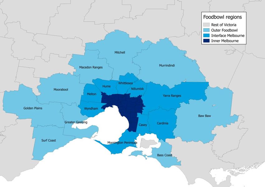
For the scope of this report, Melbourne’s foodbowl consists of the Local Government
Areas (LGAs) outlined in Table 2.1 and Figure 2.1. To highlight the different activities
between urban, peri-urban and rural areas, Melbourne’s foodbowl has been split into
three distinct regions:
• Inner Melbourne consists of the well populated LGAs that lie
predominantly within Melbourne’s urban boundary.
• Interface Melbourne consists of the LGAs that make up the edge of Greater
Melbourne, overlapping with the urban fringe.
• Outer foodbowl consists of the areas adjacent to the interface – or the
‘inner rural’ areas. Aside from Greater Geelong, these are predominantly
rural or coastal areas.
Table 2.1: Definition of foodbowl areas
Inner Melbourne Interface Melbourne Outer foodbowl
Banyule Cardinia Bass Coast
Bayside Casey Baw Baw
Boroondara Hume Golden Plains
Brimbank Melton Greater Geelong
Darebin Mornington Peninsula Macedon Ranges
Frankston Nillumbik Mitchell
Glen Eira Whittlesea Moorabool
Greater Dandenong Wyndham Murrindindi
Hobsons Bay Yarra Ranges Surf Coast
Kingston Cardinia
Knox
Manningham
Maribyrnong
Maroondah
Melbourne
Monash
Moonee Valley
Moreland
Port Phillip
Stonnington
Whitehorse
Yarra
2Figure 2.1 Map of Melbourne’s foodbowl
Source: Deloitte Access Economics
2.2 Agricultural production in the foodbowl
2.2.1 Agricultural land
As with most developed cities, agricultural land is relatively scarce in Metropolitan
Melbourne. The majority of agricultural production that feeds Melbourne’s population
takes place on the outskirts of the city and beyond, reflecting greater land availability and
less pressure from residential encroachment. Melbourne’s foodbowl accounts for more
than 1.7 million hectares, around 12% of Victoria’s 14.8 million hectares of agricultural
land. Of this, around three quarters of it is located in the Outer foodbowl, beyond the
urban boundary. Agricultural land within Greater Melbourne is located almost entirely
across interface areas, with inner Melbourne accounting for just 0.1% of Victoria’s
agricultural land (see Chart 2.1).
3Chart 2.1 Victorian agricultural land, by region
0.1% 3% Inner Melbourne
Interface Melbourne
9% Outer Foodbowl
Rest of Victoria
Victorian agricultural
land:
88% 14.8m hectares
Source: ABS Census of population and housing, mesh block counts (2010-11)
2.2.2 Agricultural Production
Agricultural production within the three foodbowl regions to an extent reflects the
availability of suitable land, with more production occurring in the outer regions (see
Chart 2.2). However, while land availability is relatively lower in Melbourne’s interface
than the outer regions, its industries produce a higher share of the total foodbowl
production than its land share would suggest.
Chart 2.2 Value of Agricultural Production in Melbourne’s foodbowl, by LGA
Baw Baw
Golden Plains
Bass Coast
Moorabool
Surf Coast
Murrindindi
Greater Geelong
Mitchell
Macedon Ranges
Cardinia
Mornington Peninsula
Whittlesea
Casey
Wyndham
Yarra Ranges
Hume
Melton
Nillumbik
Greater Dandenong
Frankston
Darebin
Kingston
Manningham
Port Phillip
Brimbank
Knox
0 50 100 150 200 250 300 350 400
$ millions (2010-11)
Inner Melbourne ($40m) Interface Melbourne ($818m) Outer foodbowl ($931m)
Source: ABS Value of agricultural commodities produced (2010–11).
4Chart 2.3 displays the main commodities produced across the three regions. Vegetables,
poultry (chicken meat and eggs), and fruit are all generally produced in greater volumes in
the inner foodbowl than they are in the outer areas, while land-intensive pastoral (cattle,
dairy and sheep) and cropping industries are more prevalent in the outer foodbowl.
Chart 2.3 Gross value of agricultural production in Melbourne’s foodbowl
Other livestock
Other crops
Eggs
Sheep
Fruit
Meat Cattle
Dairy
Poultry
Vegetables
0 100 200 300 400 500
$million (2010-11)
Outer food bowl Interface Melbourne Inner Melbourne
Source: ABS Value of agricultural commodities produced (2010-11).
2.2.3 Employment in agriculture
As at 2011, there were 12,600 people employed in all agricultural industries in
Melbourne’s foodbowl, including non-food agriculture.3 There were 9,200 people
employed (or 7, 687 when expressed as full time equivalents, or FTEs4) on-farm in major
food-producing industries (Chart 2.4).
Agriculture accounts for only a small share (0.2%) of employment in inner Melbourne,
reflecting the large concentration of jobs in service-based industries around Melbourne’s
CBD. This share is larger in the interface (2%) and outer foodbowl areas (5%). For Victoria
as a whole, agriculture accounts for 2.2% of employment.
In the outer foodbowl, the major employment industries are sheep, beef cattle and dairy
farming, while in the interface it is vegetables and fruit and nuts. Employment in poultry
farming is disproportionately low, for both eggs and meat, relative to the value of output,
reflecting greater automation and lower labour intensity in those industries.
3
Predominantly horse studs, nurseries or undefined agricultural industries
4
Deloitte Access Economics’ estimate – see Chapter 3.2
5Chart 2.4 Persons employed in agriculture in the foodbowl, food production only
Pig farming
Poultry farming - meat
Poultry farming - Eggs
Cropping
Fruit and nut
Dairy
Vegetables
Beef and Sheep farming
0 500 1000 1500 2000 2500 3000 3500
Number of employees
Outer Foodbowl Interface Melbourne Central Melbourne
Source: ABS Census of Population and Housing (2011).
Note: Excludes non-food agriculture and wine grapes that are processed on-farm. ‘Beef and sheep farming’
includes feedlots. Excludes non-food commodities such as turf and floriculture. Mixed beef/sheep/cropping
enterprises included in ‘cropping’
2.3 Food manufacturing activities
Across Melbourne’s foodbowl, the most prominent processing industries (by
employment) are dairy, meat and fruit and vegetable production. These processing
industries are likely to source primary agricultural produce from within Melbourne’s
foodbowl, as well as the rest of Victoria and Australia.
Chart 2.5 Employment in selected food processing industries, by region
Grain milling, cereal &
oil manufacturing
Poultry
Wine-making
Fruit and veg processing
Meat and smallgoods
Dairy processing
0% 2% 4% 6% 8% 10% 12% 14% 16%
Share of food processing employment
Outer Foodbowl Inner Foodbowl - interface Inner Foodbowl
Source: ABS Census of Population and Housing (2011)
Note: Excludes bakery product manufacture and other food products which process less primary produce.
Unlike primary production, downstream industries that process food are more prominent
in the inner suburbs of Melbourne, rather than the areas beyond the urban boundary. The
6main exception to that is poultry, which tends to be processed close to where chickens
are hatched and raised.5
The figures in the chart above include office-based employment in food processing
industries. A number of food processing firms, such as dairy companies, have head-offices
in Melbourne, which partially explains the relatively high proportion of employment in
inner-areas. However, food processing plants are also located across inner Melbourne’s
industrial areas.
The economic contribution of the foodbowl’s food processing sector, in terms of value
added and employment, is discussed in Chapter 3.
2.4 Food consumption in Melbourne
There is no comprehensive data source on food consumption in Melbourne. Approaches
to measuring food demand are therefore generated through multiplying population by an
estimate of per-capita consumption for Australia.
Per-capita food consumption can either be estimated by using a national accounting
approach (production less exports plus imports) or by using ABS nutritional data on the
average intake across major food groups. In this report, the second approach has been
used, following the same two-step approach adopted by the University of Melbourne’s
Victorian Eco Innovation Lab in the Foodprint Melbourne project. The broad approach is
to estimate the ‘average’ Australian diet by major food category using ABS nutritional
data, which is survey-based, and applying that average intake to the population of
Melbourne.
2.4.1 The ‘average’ Australian diet
The average Australian diet, split into major food groups, is displayed in Chart 2.6 below.
On average, Australians eat approximately 1.2 kilograms of food per day, consisting
mostly of dairy, fruit, vegetables, grains and meat.
5
Australian Chicken Meat Federation: http://www.chicken.org.au/page.php?id=3
7Chart 2.6 Average daily dietary intake, by food category
Salt
Other Seafood
Nuts
Mutton & lamb
Legumes
Rice
Fish
Oil crops
Pig meat
Eggs
Beef & veal
Chicken meat
Sugar
Cereals
Vegetables
Fruit
Dairy
0 100 200 300 400
Grams eaten per day
Source: Estimated by the Victorian Eco Innovation Lab (2016) based on data from the ABS Australian Health
Survey 2011-12
2.4.2 Melbourne’s growing population
Melbourne is Australia’s second most populated city, with around 4.6 million residents as
at June 2016 (Chart 2.7).6 According to Victorian Government projections, Melbourne’s
population is forecast to continue to grow to over 7 million people before 2050.
Melbourne’s population is expected overtake Sydney’s before then, which would see it
become Australia’s most populated city.
Assuming no changes to the average diet (while acknowledging that diets are likely to
change), Melbourne’s food demand is expected to grow in line with the population
growth displayed on Chart 2.7.
6
Greater Melbourne differs from our definition of Melbourne’s foodbowl. It largely covers Inner Melbourne,
the majority of Interface Melbourne and parts of the Mitchell LGA.
8Chart 2.7 Population of Greater Melbourne, 2011 to 2051
9
8
7
Population (million)
6
5
4
3
2
1
0
2011 2016 2021 2026 2031 2036 2041 2046 2051
Year
Source: Victoria in Future (2015) – Greater Melbourne Population
2.4.3 How much primary produce is required to feed Melbourne?
Using the population and dietary intake data above, the volume of each food commodity
required to feed Melbourne can be calculated from the product of the two. However,
wastage occurs between the farm gate and the point of consumption. For consumption
estimates to be consistent with primary production data, they must be adjusted
accordingly. Wastage can occur because:
The volume of produce that leaves the farm each day contains non-consumable
product, such as bones (for meat), stalks (for fruit and vegetables) or husks
(grain).
The processing of primary food products often results in wastage or loss of
volume.
Not all food that is prepared for sale, or sold, is consumed. Some perish on-farm
and during transportation, in supermarkets, markets, homes and restaurants.
Using data from the FAO, Sheridan et al. (2016) 7 estimated the volume of food required
at the primary stage by adjusting the volume of food consumed. These volumes allow for
‘lost’ food which is inedible or lost when food crops and livestock are harvested,
processed and/or consumed.
7
Sheridan, J., Carey, R. and Candy, S. 2016, Melbourne’s Foodprint: What does it take to feed a city?,
Victorian Eco-Innovation Lab, The University of Melbourne, available at
http://www.ecoinnovationlab.com/wp-content/attachments/Foodprint-Melb-What-it-takes-to-feed-a-
city.pdf
9For each food group, these adjusted volumes of food required to feed Melbourne at its
current population (4.6 million) and in future (7 million), are displayed in Chart 2.8,
together with 2011 production levels for Melbourne’s foodbowl and the rest of Victoria.
Chart 2.8 Melbourne’s food demand now and in future (thousand tonnes)
Note: Victorian production of milk and cereal grains exceeds 3,000 kilo tonnes (and the scale of this chart).
Chart 2.8 demonstrates that foodbowl production is insufficient to meet current
estimated food demand for all agricultural commodities except for eggs and poultry meat.
Vegetable production in the foodbowl is equivalent to over 80% of Melbourne’s
consumption, suggesting that local production could potentially meet most, but not all of
Melbourne’s fresh vegetable demand. However, due to factors such as those listed in
section 2.4.4 (below), it is likely that not all food produced in Melbourne’s foodbowl is
consumed there.
At the state level, Victorian production exceeds Melbourne’s estimated demand for each
commodity group except for sugar, rice and pig meat. Production of some of Victoria’s
major export commodities (cereals, milk, beef and sheep meat) significantly exceeds
Melbourne’s demand.
2.4.4 How much of Melbourne’s food is locally sourced?
Estimating the proportion of Melbourne’s foodbowl production that is consumed locally is
largely an assumption-driven exercise, aided by a limited body of research and supporting
data. 8 9 10 In addition, the contracts between growers, processors, wholesalers and
retailers which would determine how food moves around the state are not made public.
8
Timmons, D., Q. Wang and D. Lass 2008, Local Foods: Estimating Capacity, Journal of Extension, vol 46 (5),
available at http://www.joe.org/joe/2008october/a7.php
10While comparing likely local consumption with local agricultural production can
demonstrate the likelihood that certain foods are sourced locally, there are other factors
to consider, including:
• Perishability and freshness: Food that perishes easily is more likely to be
locally sourced than that which can be stored for longer periods. For
example, poultry meat has a relatively short shelf life (unless frozen), while
rice and other grains can be stored for years without perishing.
• Seasonality: Where there is year-round demand, perishable fruit and
vegetables that are in season for short windows must be sourced from
elsewhere at various times throughout the year. Berries and capsicums are
two examples – Victorian producers will send produce north when in
season, while northern producers will meet Melbourne’s demand for part
of the year. The share of locally sourced food consumed therefore varies
throughout the year, which is not captured in annual
production/consumption data.
• Definition of local: How businesses and consumers define ‘local’ can be
subjective. For some, locally grown food can mean it was grown in the
same country or the same state, while for others, the size of the radius
which implies something is ‘local’ can be much smaller. Food produced in
the foodbowl can enter bulk supply chains which span the state, other parts
of the country, and can still be branded as ‘local’.
• Traceability: Even when local branding carries value, products that are
highly commoditised are not easily traceable once pooled with produce
from across the state and country. Cereal grains are one such example. This
is in contrast with some horticulture, meat and eggs, where the origin can
be easily communicated to consumers.
Applying these factors across a range of commodities, and informed by some consultation
with industry, Deloitte Access Economics has developed a set of assumptions on how
much of the foodbowl’s agricultural production is consumed locally. For the purpose of
this analysis, local food is defined as food produced in Melbourne’s foodbowl that is
consumed within the foodbowl region (which includes Greater Melbourne and outer
foodbowl LGAs). These assumptions are outlined in Appendix C. While informed by data,
these assumptions are only estimates to be used in the modelling that is discussed in
Chapters 3 and 4.
9
Conner, D., F. Becot, D. Hoffer, E. Kahler, S. Sawyer and L. Berlin 2012, Measuring current consumption of
locally grown foods in Vermont: Methods for baselines and targets, Journal of Agriculture, Food Systems and
Community Development, available at http://mainefoodstrategy.com/wp-
content/uploads/2013/05/jafscd_measuring_local_food_consumption_vermont_may-2013.pdf
10
Masi, B., L. Shaller and MH. Shuman 2010, The 25% shift: the benefits of food localization for Northeast Ohio
& how to realise them.
113 Economic contribution of
Melbourne’s foodbowl
Deloitte Access Economics has estimated the economic contribution of Melbourne’s
foodbowl. The estimation provides a snapshot of the economic footprint of agriculture and
related value-adding activities in Melbourne’s foodbowl throughout the regional economy.
This chapter describes the methodology and assumptions (section 3.1) and presents the
results of the analysis (section 3.2).
3.1 Methodology
There are two parts to the economic contribution of Melbourne’s foodbowl; its direct
contribution and its indirect contribution.
The direct contribution of an industry is measured as the value added by the
activities of businesses within that industry, which is the sum of returns to labour
and capital. Value added is a commonly adopted metric used to measure the
economic contribution of industries and sub-sectors. This study measured the
direct contribution of the agriculture and food manufacturing sectors in
Melbourne’s foodbowl.
The indirect contribution of an industry is measured using Input-Output (IO)
modelling. The linkages and interdependencies between various sectors of an
economy are observed and used to analyse which outputs represent final demand
and which flow to other sectors as inputs. The linkages between sectors are
published by the ABS in the national accounts data.
Regional Input-Output model
Deloitte Access Economics has used the Global Trade Analysis Project (GTAP) input-output
tables, which are based on the ABS national input-output tables, with the additional
breakdown of agriculture into sub-sectors, including vegetable, poultry, and dairy
production. Deloitte Access Economics then developed a regional-level IO model for
Melbourne’s foodbowl with the following additional data:
• ABS 2011 census working population profile data (place of work) – used to infer
regional production and consumption. In this case, agricultural production and
consumption were inferred using sourcing assumptions outlined in appendix C.
• National import data - used to determine what is flowing into the region
• Trade flows between regions using local sourcing assumptions, which reflect that
regional demand is met by local supply, distant supply and imports (see Section
2.4.4).
More details are provided in Appendix A.
123.2 Results
3.2.1 Economic contribution of agriculture and related value-
adding activities in Melbourne’s foodbowl
The total economic contribution of agriculture to the regional economy, including
upstream and downstream activities, is estimated to be around $2.45 billion per annum
(in 2014–15 dollars, see Table 3.1). The agriculture sector also generates 21,001 full time
equivalent (FTE) jobs in the region.11 This represents 0.84% of the entire Melbourne
regional economy, and 1.06% of its work force.
This total contribution can be split into three distinct categories: direct contribution of the
agriculture sector (from on-farm activity and employment), indirect contribution (through
expenditure in sectors generating inputs to the agriculture sector), and direct contribution
of food manufacturing (downstream to the agriculture sector):
The agriculture sector directly contributes approximately $956 million per annum
in value-added terms to the regional economy and directly employs 7,687 people
on a full time equivalent (FTE) basis.
Agriculture’s indirect contribution, reflecting expenditure on intermediate inputs
(such as water, machinery, feed, fertiliser and seed), includes $742 million per
annum in value-added terms, and 5,719 FTEs employed in upstream sectors that
provide inputs into the sector.
Food manufacturing in the region, which uses the agricultural produce grown
within the foodbowl, contributes a further $756 million per annum to the regional
economy and employs 7,595 FTEs directly.
Table 3.1 Economic contribution of agriculture and food manufacturing in Melbourne’s
foodbowl
Agriculture Food Total agri-food
manufacturing contribution
Direct Indirect Direct
Value added ($million) 956 742 756 2,454
Employment (FTEs) 7,687 5,719 7,595 21,001
Source: Deloitte Access Economics. Note that value added figures are denoted in 2014-15 dollars.
Agriculture’s direct economic contribution in both value-added and employment terms is
only slightly higher than its indirect contribution. This is because agriculture’s expenditure
on intermediate inputs (such as water, machinery, feed, fertiliser and seed) is relatively
high.
11
Employment expressed in FTE’s is typically lower than when expressed as jobs, as it is in Chapter 2.
133.2.2 Sectoral economic contribution
The sectoral economic contribution is presented in Table 3.2. Fruit and vegetables’ direct
contribution to the regional economy in value-added terms is the highest at 43% of
agriculture’s total direct contribution ($413 million per annum), followed by other animal
products12 at 20% ($201 million per annum) and livestock 13 at 17% ($163 million per
annum). For indirect value added, the ordering is slightly different with other animal
products ranked the highest ($290 million), followed by fruit and vegetables ($151 million)
and livestock ($145 million).
Table 3.2 Sectoral economic contribution in Melbourne’s foodbowl
Value added ($ million) Employment (FTEs)
Commodity group Direct Indirect Direct Indirect
Food crops 43 23 403 163
Vegetables and Fruits 413 151 2997 1,052
Livestock 163 145 1493 1,107
Other animal products 201 290 1537 2,387
Dairy 137 134 1257 1,011
Total 956 742 7,687 5,719
Source: Deloitte Access Economics
Fruit and vegetables also directly employ the largest number of people in agriculture in
the foodbowl. Their direct contribution in employment terms is the highest at 39% (2,997
FTEs) of total number of people directly employed in agriculture. Other animal product
industries create the highest indirect contribution in employment term (2,387 FTEs). This
indicates that other animal industries in the foodbowl source inputs from upstream
industries that are relatively labour-intensive.
12
Defined as eggs, pigs and poultry
13
Beef, sheep and goats
144 Economic impacts under
alternative future scenarios
In this chapter, the economic impacts of changes in land use from agricultural production
to urban development to accommodate Melbourne’s 7 million people and changes in
preference of consumers in Melbourne’s foodbowl for more locally grown food are
estimated. This chapter describes the methodology and assumptions (section 4.1) and
presents the results of the economic impact analysis under these changes (sections 4.2 and
4.3).
4.1 Methodology
This project utilises the Deloitte Access Economics – Regional General Equilibrium Model
(DAE-RGEM). DAE-RGEM is a large scale, dynamic, multi-region, multi-commodity CGE
model of the world economy that encompasses all economic activity in an economy –
including production, consumption, employment, taxes and trade – and the linkages
between them. For this project, the model has been customised to explicitly include
Melbourne’s foodbowl regional economy and its unique economic characteristics.
Figure 4.1 The components of DAE-RGEM and their relationships
Figure 4.1 is a stylised diagram showing the circular flow of income and spending that
occurs in DAE-RGEM. To meet demand for products, firms purchase inputs from other
producers and hire factors of production (labour and capital). Producers pay wages and
rent (factor income) which accrue to households. Households spend their income on
goods and services, pay taxes and put some away for savings. The government uses tax
revenue to purchase goods and services, while savings are used by investors to buy capital
goods to facilitate future consumption. As DAE-RGEM is an open economy model, it also
15includes trade flows with other regions, states, and foreign countries. More details are
provided in Appendix B.
Because Melbourne’s foodbowl is not explicitly represented in the database underlying
DAE-RGEM, we customised the spatial regions of the model. Melbourne’s foodbowl
consists of the Local Government Areas (LGAs) outlined in Table 2.1 and Figure 2.1.
In the following sections, the description of the scenarios and their results are discussed.
4.2 Melbourne growing to accommodate 7
million people
The study compares a baseline scenario of existing Melbourne land use to two alternative
scenarios that reflect two alternative ‘sprawl’ scenarios where land currently used for
agriculture is developed to accommodate a population of 7 million people, which is
expected to occur between 2041 and 2046. 14
The baseline scenario reflects the existing current land use profile of Melbourne’s
foodbowl area. In order to isolate the effects of land use changes in each of the
scenarios, population (which drives food demand) is held constant at 7 million
people in the base case and the two scenarios.
The alternative scenarios, ‘constrained urban sprawl’ and ‘moderate urban
sprawl’, reflect alternative ways in which Melbourne could grow to accommodate
future population growth. The ‘constrained urban sprawl’ scenario represents a
situation where less land is required for residential development than the
‘moderate urban sprawl’ scenario. The different rates of agricultural land
retention reflect different assumptions about both the future density of existing
residential areas (infill) and new housing developments. The assumptions driving
each alternative scenario are summarised in Table 4.1.
Table 4.1 Assumptions under alternative growth scenarios
Commodity group Constrained Moderate
urban sprawl urban sprawl
scenario scenario
Population growth (additional people) 2.4 million 2.4 million
Infill rate (%) 79% 61%
Average site density in new areas (lots per hectare) 25 15
Gross density in new areas (dwellings per hectare) 15.5 9.3
Persons per dwelling 2.95 2.95
Additional dwellings required in growth (number) 169,000 314,000
Land required for new developments (hectares) 10,897 33,730
Note: Gross density includes surrounding open space, commercial properties and infrastructure required in
new development areas. Site-to-gross density was calculated from the average of ten new residential sites.
14
Victoria in Future (2015)
16The assumptions presented in Table 4.1 have been informed by previous studies on
Melbourne’s development. Buxton et al. (2015)15 estimated that an infill rate of around
79% could be achieved in Melbourne out to 2050. In other words, 79% of population
growth could be accommodated by residential development within existing urban areas,
with the remaining 21% developed in growth areas. It is worth noting that the infill rate of
79% is an aspirational goal. Plan Melbourne (2014) has a projected infill rate of 61%.
These two alternative infill rates have been used in the ‘constrained urban sprawl’ and
‘moderate urban sprawl’ scenarios, respectively.
Assuming that dwellings in new developments will contain, on average, 2.95 people 16,
there will be 169,000 additional dwellings required in growth areas under the
‘constrained urban sprawl’ scenario and 314,000 additional dwellings required in growth
areas under the ‘moderate urban sprawl’ scenario.
The average densities in the two scenarios are based on current guidelines for medium
(25 per hectare) and low (15 per hectare) lot densities in new residential developments.17
Assuming (on average) high density developments, there will be approximately 11,000
hectares converted from agricultural land to residential land in the ‘constrained urban
sprawl’ scenario. Assuming medium density development occurs, the equivalent area is
around 34,000 hectares in ‘moderate urban sprawl’ scenario.
To estimate the impact on agricultural industries, the agricultural land impacted by the
growth has been apportioned to the growth corridors within Melbourne’s seven growth
LGAs (Hume, Mitchell, Melton, Wyndham, Casey, Cardinia and Whittlesea), according to
forecast population growth to 2031 (Table 4.2).
Table 4.2 Residential growth and agricultural land in 9 growth LGAs
Local Government Area Share of population Agricultural Land Agricultural Production
growth in new (Ha, 2011) ($m, 2011)
residential areas
Cardinia Shire 9% 108,465 290
City of Casey 18% 17,933 114
City of Hume 10% 15,509 12
City of Melton 16% 7,645 8
Mitchell Shire 6% 108,765 44
City of Whittlesea 17% 10,174 108
City of Wyndham 24% 16,429 86
Source: ABS Mesh Block counts, Victoria in Future (2015). ABS Value of Agricultural Commodities Produced
2010-11 (cat. 7503.0). Growth areas (VIFSAs) include: Koo Wee Rup, Officer-Pakenham, Cranbourne, Bulla-
Craigieburn, Caroline Springs-Hillside, Rockbank, Kilmore-Wallan, Epping-Whittlesea, Hoppers Crossing-
Truganina, Point Cook-Werribee South, and Werribee-Wyndham Vale.
15
Buxton, M., J. Hurley and K. Phelan 2015, Melbourne at 8 million: matching land supply to dwelling demand,
Centre for Urban Research, RMIT University, October.
16
Population–weighted average of seven growth LGAs. Source: ABS Census of population and housing (2011)
17
Within new urban developments, densities typically range from 15 lots to 25 lots per hectare, as outlined in
Precinct Structure Plans released by the MPA. See: http://www.mpa.vic.gov.au/planning-
activities/greenfields-planning/precinct-structure-plans/
17It is important to note that if land is not used for urban dwelling development, the
assumption is that it would be used for agricultural production. In other words, other
alternative uses for this land are not modelled.
4.2.2 Constrained urban sprawl – results
Table 4.3 presents the sectoral impacts of Melbourne’s population increasing to 7 million
and urban sprawl being constrained, compared to the land use profile in the baseline.
Table 4.3 Sectoral impacts of ‘constrained urban sprawl’
Commodity group Output Output Employment Employment Price
($m) (%) (FTEs) (%) change (%)
Agriculture -32 -0.4316% -70 -0.296% 0.324%
Mining 6 0.0077% 4 0.007% -0.001%
Food manufacturing -11 -0.0232% -18 -0.016% 0.013%
Other Manufacturing 2 0.0011% 10 0.002% -0.002%
Water/Waste/electricity 0 -0.0013% 0 0.001% -0.002%
Transport -6 -0.0045% -8 -0.003% -0.003%
Construction -1 -0.0019% 0 0.000% -0.003%
Services -19 -0.0024% -26 -0.001% -0.003%
Total -62 -0.0047% -107 -0.003% 0.000%
Source: Deloitte Access Economics
Impact on agriculture
As shown in Table 4.3, compared to the baseline scenario, a reduction in agricultural land
of 10,897 hectares would lead to a reduction in annual agricultural output of $32 million
(0.43%). This leads to a loss in agricultural value-add of over $10 million. As long as the
scenario holds, this annual impact is ongoing in perpetuity. Agricultural employment, as a
consequence, will be 70 FTEs lower than in the baseline. Also reflecting the greater
scarcity of agricultural land, the farmgate price of agricultural produce, are expected to be
0.3% higher than the baseline.
Impact on food manufacturing and the regional economy
Food manufacturing is a downstream sector of agricultural production. As a result of
declining agricultural output, food manufacturing’s annual output will decrease by $11
million (0.023%) under the constrained urban sprawl scenario, relative to the baseline
scenario. As previously discussed, as long as the scenario holds, this impact on food
manufacturing’s output is ongoing in perpetuity.
Reflecting a lower level of output in food manufacturing, employment in this sector in
Melbourne’s foodbowl will decrease by 18 FTEs compared to the baseline scenario.
Compared to the 7,595 FTEs directly employed in food manufacturing in Melbourne’s
foodbowl, this amount appears modest, however the impact could be concentrated to
particular areas depending on the agricultural land affected.
18Similarly, the price of processed foods is expected to increase under the scenario,
reflecting a reduction in Melbourne’s food supply. It is estimated that prices of these
products will be 0.013% higher than the baseline (Table 4.3).
As a result of declining agricultural output, there are other flow-on effects to the rest of
the economy (see Table 4.3). In particular, the economy’s annual output falls by $62
million (0.0047%), leading to a reduction in the GRP of Melbourne’s foodbowl of $35
million and a decrease in regional employment of 107 FTEs, relative to the baseline
scenario.
Overall, the annual impacts on the regional economy appear to be modest. However, the
cumulative impacts of this scenario could be significant. As long as the same impacts on
gross regional product18 (GRP) occur every year from, for example, 2050 to 2070, the net
present value of the cumulative impact would be $376 million (in 2014–15 dollars). It is
noted this estimate represents a best case scenario, because as population continues to
grow, urban development will also continue.
4.2.3 Moderate urban sprawl – results
Table 4.4 presents the sectoral and price impacts of Melbourne’s population increasing to
7 million and urban sprawl occurring at a faster rate under the second of the two
alternative scenarios.
Table 4.4 Sectoral impacts of ‘moderate urban sprawl’
Commodity group Output Output Employment Employment Price
($m) (%) (FTEs) (%) change (%)
Agriculture -111 -1.49% -240 -1.02% 1.13%
Mining 21 0.03% 14 0.02% 0.00%
Food manufacturing -38 -0.08% -62 -0.06% 0.04%
Other Manufacturing 8 0.00% 36 0.01% -0.01%
Water/Waste/electricity -1 0.00% 1 0.004% -0.01%
Transport -21 -0.02% -29 -0.01% -0.01%
Construction -5 -0.01% 0 0.00% -0.01%
Services -70 -0.01% -95 -0.003% -0.01%
Total -217 -0.02% -375 -0.009% 0.00%
Source: Deloitte Access Economics
Impact on agriculture
The impact of the ’moderate urban sprawl’ scenario would lead to a reduction of annual
agricultural production of $111 million (1.49%), relative to the baseline scenario. This
leads to a loss in agricultural value-add of around $35 million. Agricultural employment
will be 240 FTEs lower. The reason that the economic impacts on agriculture would be
higher in this scenario than in the ‘constrained urban sprawl’ scenario is that less
18
Gross regional product refers to the annual output of a regional economy, just as gross domestic product
(GDP) refers to the annual output of a national economy
19constrained urban sprawl would lead to more agricultural land loss, hence, a bigger loss to
agricultural output.
Also reflecting the greater scarcity of agricultural land, the farmgate prices of agricultural
products grown in the foodbowl are expected to be 1.13% higher than prices in the
baseline. This impact is more than 3 times higher than the equivalent impact when urban
sprawl can be constrained, reflecting the greater value of these agricultural products.
Impact on food manufacturing and the regional economy
Table 4.4 also shows the impact of less constrained urban sprawl on food manufacturing,
relative to the hypothetical base case. As a result of declining agricultural output, food
manufacturing’s output will be $38 million (0.08%) lower than the base case. Employment
in food manufacturing in Melbourne’s foodbowl would reduce by 62 FTEs, relative to the
base case, due to the lower level of output.
Similarly, prices of processed foods are expected to be 0.04% higher than the base case,
reflecting a relatively larger reduction in Melbourne’s food supply (Table 4.4). The
increase in prices of processed foods largely reflects the higher input costs to food
manufacturing as agricultural produce becomes more expensive.
There are also other flow-on effects to the rest of the economy (Table 4.4). Overall, the
annual impact on the regional economy is larger than that in the ‘constrained urban
sprawl’ scenario. In particular, the economy’s annual output will fall by $217 million
(0.02%) relative to the base case, leading to a reduction in GRP of Melbourne’s foodbowl
of $122 million (compared to $35 million in ‘constrained urban sprawl’ scenario). Regional
employment will be 375 FTEs lower. This loss is more than 3 times that of the equivalent
impact in the previous scenario.
The cumulative impact on GRP of this scenario could be significant. As long as the same
impact on GRP occurs every year over a 20 year period in the future (say, 2050 to 2070)
the net present value of the cumulative decrease in GRP under this scenario would be
about $1.33 billion (in 2014–15 dollars). As noted previously, this represents a best case
scenario because population growth and urban development will likely continue.
4.2.4 Discussion
The result from the two urban sprawl scenarios highlights how accommodating
Melbourne’s growing population will result in a loss of agricultural land at varying
degrees, reducing output and employment in both the agricultural and food
manufacturing industries. Comparing the results of the two scenarios shows how the
negative economic impacts on GRP and employment, could be minimised by constraining
urban sprawl, primarily through retaining agricultural land. If population is growing
according to current trends, expanding urban sprawl would lead to significant negative
impacts on these measures in the future.
At the sectoral level, the negative impacts on agriculture and food manufacturing are the
result of the loss in agricultural land, hence, agricultural output. Lower food supply
resulting from less available agricultural land would likely lead to higher farmgate prices
for primary produce, and higher prices for processed foods. These price increases would
20You can also read