The Impact of Home Sharing on Residential Real Estate Markets - MDPI
←
→
Page content transcription
If your browser does not render page correctly, please read the page content below
Journal of
           Risk and Financial
           Management

Article
The Impact of Home Sharing on Residential Real
Estate Markets
Helen X. H. Bao *         and Saul Shah
 Department of Land Economy, University of Cambridge, Cambridge CB3 9EP, UK; Sps57@cam.ac.uk
 * Correspondence: hxb20@cam.ac.uk

 Received: 18 June 2020; Accepted: 22 July 2020; Published: 25 July 2020

 Abstract: This paper explores the effects of home-sharing platforms in general and Airbnb in
 particular on rental rates at a neighbourhood level. Using consumer-facing Airbnb data from ten
 neighbourhoods located within large metropolitan areas in the U.S. between 2013–2017, as well as
 rental data from the American online real estate database company, Zillow, this paper examines the
 relationship between Airbnb penetration and rental rates. The results indicate that the relationship is
 not as unanimous as once thought. Viewing the relationship at an aggregate level, an approach used
 by many researchers in the past, hides the complexities of the underlying effects. Instead, Airbnb’s
 impact on rental rates depends on a neighbourhood’s individual characteristics. This study also urges
 policy makers to create tailor-made solutions that help curb the negative impacts associated with the
 platform whilst still harnessing its economic benefits.

 Keywords: sharing economy; time series analysis; random effect panel model; rents

1. Introduction
     The sharing, or gig-economy, defined here as a series of platforms that facilitate ‘the peer-to-peer-based
activity of obtaining, giving, or sharing the access to goods and services’ (Hamari et al. 2016, p. 2047)
has seen tremendous rates of growth in the past decade and has now become an integral part of our
everyday lives. Predictions made by PricewaterhouseCoopers suggest that this economy could grow
to generate more than $335 bn of revenue worldwide by 2025, up from the $14 bn it created in 2014
(Matzler et al. 2015). At the forefront of this booming economy sits Airbnb, a platform that looks to
transform the way in which we utilise our most valuable asset: housing. The platform, which has
now become a household name, looks to connect short-term tenants with various types of landlords in
an effort to provide a more authentic travel experience to visitors whilst generating economic profits
for suppliers.
     The success of Airbnb can be seen in numbers: it now advertises over 7 million listings and
operates in 191 countries around the world (Airbnb Newsroom 2020). Despite the size of the platform,
very little is known about Airbnb and its impact on real estate markets. Existing studies on the effect
of Airbnb establishment in the neighbourhood on housing prices are very limited in terms of the
geographic areas covered (Zou 2020). Additionally, Airbnb takes great pain in hiding its operations
from public view, leading to numerous accusations of tax evasion and an expanding list of third
parties taking legal action against the platform. It even creates political tensions and is becoming a
hotly debated area in urban development (McNeill 2016). These recent developments make it more
important than ever to identify the platform’s effects in order to better check its future growth.
     Despite the recent criticism, Airbnb, and the sharing economy as a whole, is argued to generate a
multitude of economic benefits. It is theorised that the short-term exchanges allow for better resource
allocation and utilisation, thereby increasing both the productivity and efficiency of the economy
(Jevons 2015). The platforms also lower the barriers to entry in many markets, allowing more users

J. Risk Financial Manag. 2020, 13, 161; doi:10.3390/jrfm13080161                     www.mdpi.com/journal/jrfm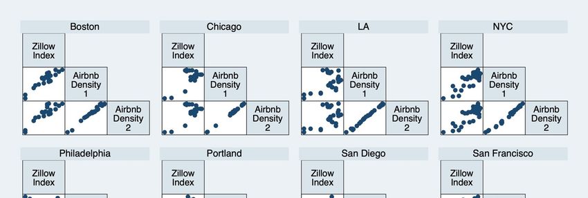
J. Risk Financial Manag. 2020, 13, 161                                                              2 of 18

to list their offerings of goods and services. Furthermore, in the case of Airbnb, the newly generated
rental income received by local landlords, as well as the additional spending by tourists, can benefit
neighbourhood restaurants and shops, increasing the level of wealth within an area and improving the
amenities and services available to local residents.
      Nevertheless, many argue that the expansion of Airbnb has brought with it many drawbacks.
Firstly, academics theorise that the increase in rental income offered by Airbnb has led to landlords
switching to the short-term market in order to profit from tourist demand (Barron et al. 2020). This then
decreases the supply of available housing for local residents, which increases rents and exacerbates
the already dramatic affordability issue present in many urban centres. Additionally, research has
found that that a growing proportion of listings on the platform are owned and run by profit-seeking
commercial operators. Corporations and wealthy landlords have been able to gain from the expansion
of Airbnb at the expense of tenants, thereby exaggerating the divergence between social classes around
the world.
      The objective of this study is to expand upon the limited existing literature on home-sharing in
two main ways. Firstly, the paper will look to isolate the impact that Airbnb has on rents. The analysis
will be centred around ten neighbourhoods in some of the largest metropolitan areas in the U.S. and
will involve using multiple time-series datasets covering Airbnb listings from 2013 to 2017 and a
corresponding set of indexed rental rates in order to test the primary hypothesis that increased Airbnb
densities will induce a rise in rental rates at a neighbourhood level. Secondly, the study will use the
previously mentioned analysis to investigate viable and effective policy measures that can help curb the
negative consequences associated with Airbnb whilst simultaneously harnessing its economic benefits.
      The rest of this paper is structured as follows. Section 2 begins by defining what the sharing
economy is before analysing its main characteristics and factors of growth. The literature review then
focuses on Airbnb’s demand and supply side effects and evaluates previous empirical investigations.
Section 3 lays out the methodology and datasets used in this analysis, Section 4 presents results and
outlines a discussion, Section 5 considers policy implications, and in Section 6, conclusions are made.

2. Literature Review

2.1. The Sharing Economy
      Airbnb, and home-sharing platforms more generally, operate within the broader sharing economy.
Whilst the sharing economy is a term often used to describe a number of different platforms, it is best
defined as a ‘set of peer-to-peer online marketplaces that facilitate matching between demanders and
suppliers of various goods and services’ (Barron et al. 2020, p. 2). Common examples of platforms that
operate within the sharing economy include Airbnb, Uber, HomeAway, Lyft, Deliveroo, Fiverr, Doordash,
and TaskRabbit. Despite the economy spanning such a vast range of industries, each characterised by
different features, the platforms often share common components. On all platforms, the suppliers of
products and services look to share excess capacity that might otherwise go underutilised with people
that want to use them for a short period of time (Ferreri and Sanyal 2018). Additionally, the platforms do
not own any of the assets that they are advertising, but instead facilitate sharing between participants
for a fee, often relying on spot-transactions rather than long contracts (Einav et al. 2016; Proserpio and
Tellis 2017). With many of the marketplaces being app-based, developers often utilise advancements in
technology to improve the matching between buyers and sellers and have implemented reputation and
rating systems in order to create a sense of trust on the platforms (Einav et al. 2016). In theory, there
are two main segments that operate in the ‘pure’ peer-to-peer economy. The first are decentralised
platforms. These are services that bridge the gap between demanders and suppliers, but leave the
searching, matching, and price setting to the participants (Proserpio and Tellis 2017). Examples in
this segment include Airbnb, Stashbee, and TaskRabbit. On the other hand, centralised platforms
take control and centrally match buyers and sellers, setting prices using tested algorithms. Examples
include Uber, Lyft, and Doordash.
J. Risk Financial Manag. 2020, 13, 161 3 of 18
The sharing economy, which is projected to generate more than $335 bn of revenue worldwide
by 2025, has seen tremendous growth in recent years and is rapidly changing the ways in which
we consume products and services (Proserpio and Tellis 2017). There are numerous reasons as to
why this growth has occurred. Firstly, the 2008/09 financial crisis left many without steady incomes
or employment opportunities and created a group of people that were unable to pay for assets and
services. The sharing economy thus created an opportunity for these groups to turn to alternative
platforms that compensated them for providing underused assets. Additionally, the flexibility of these
platforms allows users to decide between working on these marketplaces full-time or to use it as
a supplement to their regular income. Secondly, a wave of technological advancements, including
smartphones, apps, and WiFi has allowed for greater connectivity and has reduced search costs and
the time it takes to connect buyers and suppliers. Finally, globalisation has blurred the lines between
local and global economies. This has meant that resources that are underutilised in a local economy
can now be accessed by users on a global scale (Proserpio and Tellis 2017).
The sharing economy is celebrated by many as an innovation that improves economic efficiencies
by reducing the frictions caused by excess capacity whilst also being capable of disrupting established
industries (Barron et al. 2020; Proserpio and Tellis 2017). Proponents of these marketplaces applaud
the platforms’ ability to provide consumers with a better matching and use of resources, lower prices,
better offerings, and an overall increase in welfare (Barron et al. 2020). Additionally, the economy’s
flexibility mentioned previously is argued to foster micro-entrepreneurialism as individuals are
able to monetise their assets whilst still contributing to the GDP through their regular occupations
(Ferreri and Sanyal 2018). This being said, however, there are many that argue that these platforms’
negatives outweigh their benefits. More specifically, recent evidence has shown that the sharing
economy may increase societal inequality (Schor 2017) and lower city centre affordability whilst
displacing lower income populations to nearby communities (Lee 2016). Furthermore, academics,
including Ferreri and Sanyal (2018), contend that the sharing economy has moved away from a forum
that allows the exchange of goods and services and towards one where ‘venture capital firms come to
intervene and influence these processes’ (p. 3357).
2.2. Airbnb and Short-Term Rentals
After renting out air mattresses on their apartment floor to attendees of a conference in
San Francisco, Brian Chesky and Joe Gebbia founded Airbnb in 2008, which is now recognised
as the pioneer of not just the home-sharing industry, but the sharing economy as a whole. Airbnb
operates as a peer-to-peer marketplace for short-terms rentals, connecting tourists with suppliers of
various kinds of accommodations. It is important to note that in most academic literature, short-term
rentals (STRs) are defined as ‘lettings of up to 30 consecutive days’ (Koster et al. 2018, p. 8). The website
allows its users to advertise three different types of listings: a shared room, a private room, or an
entire unit. Local authorities and academics often distinguish between two types of short-term rentals.
‘Home-sharing’, which includes Airbnb’s shared and private room listings, is usually defined as a STR
where at least one of the primary residents lives on-site during the tourists’ stay. ‘Vacation rentals’,
on the other hand, are where the tourist occupies the entirety of the letting (Koster et al. 2018). Seeing
as Airbnb operates in both segments, the platform has essentially created a new category of rental
housing which blur the lines between traditional rentals and hotel accommodation.
Furthermore, the platform’s business model is simple: hosts list their offerings on the marketplace
for a price set by themselves, while Airbnb takes a commission of anywhere from 7% to 18% per
booking (Wachsmuth and Weisler 2018). This being said, Airbnb takes great pains in order to hide its
operations from public view and has been claimed to bypass regulations and ‘undermine policies aimed
at protecting the supply of affordable housing’ (Wachsmuth and Weisler 2018, p. 5). It is often argued
that Airbnb has moved away from a sharing platform to one that incentivises large scale operators to
accumulate additional properties in search for profit. For example, in Los Angeles, researchers found
that these large-scale property developers earn huge revenues; just 6% of hosts list more than oneJ. Risk Financial Manag. 2020, 13, 161 4 of 18
property and yet they earn 35% of all Airbnb revenue (Lee 2016). DiNatale et al. (2018) surveyed the
Airbnb markets in 237 cities in Oregon, USA. They found that nearly 40% of Airbnbs are whole homes
that are rented more than 30 days in a year, which potentially has significant impacts on long-term
rental supply in those cities.
Airbnb’s rapid growing in many cities raised serious concerns in a wide range of areas such as
anti-social behaviour (noise, disruption), public health, safety, fire risk, availability and affordability
of permanent rental housing, impacts on local services and tax revenue, and impacts on the tourism
industry (Gurran and Phibbs 2017; Gurran et al. 2018). Although Airbnb position itself as the poster
child of sharing economy by providing temporary supplies to the tourism sector, evidence is found that
Airbnb actually removes residential units from housing market permanently (Crommelin et al. 2018;
Schäfer and Braun 2016; Vinogradov et al. 2020). There are growing concerns about Airbnb’s role in
the financialization of housing (Cocola-Gant and Gago forthcoming; Grisdale 2019), displacement
(Cocola-Gant and Gago forthcoming; Yrigoy 2019), and tourism-led gentrification (Robertson et al. 2020;
Wachsmuth and Weisler 2018).
Despite these criticism and concerns, Airbnb has seen tremendous rates of growth since its
incubation in 2008. Airbnb now has over seven million properties on its platform, listed by over two
million hosts in 81,000 cities and 191 countries worldwide, more than twice as many as its closest
competitor, HomeAway (Airbnb Newsroom 2020; Barron et al. 2020; Wachsmuth and Weisler 2018).
Additionally, Airbnb has provided accommodation to over 500 million guests, allowing it to gain a
monopolistic position in many of the cities in which it operates (Airbnb Newsroom 2020; Ferreri and
Sanyal 2018). Despite attempts at regulation in order to protect local markets and curb Airbnb’s growth
(Cassell and Deutsch forthcomin), these numbers are still expected to rise. While Airbnb has yet to
have its IPO, the platform’s market penetration and profitability figures has resulted in a valuation of
over $31 bn, making it larger than some of the World’s leading accommodation chains including the
Marriot and Hilton groups (Proserpio and Tellis 2017).
2.3. The Effects of Airbnb on Rental Real Estate Markets
It is often theorised that Airbnb has two competing effects on local rental property markets.
On the one hand, the extra rental income earned by local residents is argued to enable some citizens
to continue living in ‘booming’ housing markets. On the other hand, the high revenues earnt from
short-term rentals mean that property owners of all types have an incentive to shift their supply from
the long-term market to the tourist market, which increases rents for long-term tenants. In support of
the latter argument, recent research by academics in both Europe and the USA have found that Airbnb
often distorts rental markets through either a supply effect or a demand shift.
Perhaps the leading theory on Airbnb’s effect on residential markets is that the expansion of the
platform has caused a supply shift from the long-term to the short-term rental market, decreasing total
supply in the long-term and increasing rents for local tenants. Academics suggest that the market for
long and short-term rentals is segmented on both the demand and supply side. This segmentation is
argued to exist for many reasons. On the demand side, tenants will have different needs depending on
the length of their stay: the potential tenants of short-term accommodation are usually tourists, business
travellers, and other visitors who may only be looking for a bed and bathroom. Local residents seeking
a more comprehensive dwelling, on the other hand, create the demand for long-term accommodation
(Barron et al. 2020). On the supply side, there may be legal restrictions which do not allow for the
transfer of accommodations from different term structures; additionally, landlords may prefer one
length of letting to another or may be unable to switch due to contractual obligations.
This segmentation has created a term structure of rents, with the rents coming from short-term
accommodation typically being much higher than the rents coming from long-term lettings. The gap
between the two term structures is often referred to as the ‘home-sharing premium’. The expansion of
home-sharing platforms like Airbnb have reduced the frictions between the two segments and has
allowed for the transfer of accommodation from the long-term to the short (Horn and Merante 2017).J. Risk Financial Manag. 2020, 13, 161 5 of 18
Furthermore, seeing as the supply of housing is fixed or highly inelastic in the short-run, this transition
results in a decreased supply of long-term rental properties and puts tourists in direct competition
with local renters, raising prices for all long-term accommodations (Lee 2016). This issue is exacerbated
by the fact that, in many cities, both private and public developers are already unable to build enough
new homes for their residents.
There is substantial evidence that a supply side factor has contributed to the rising rental prices in
many cities. Focusing on U.S. metropolitan areas, Barron et al. (2020) engaged in regression analysis
to discover a causal relationship between Airbnb penetration and rental rates. More specifically,
they found that, on average, a 1% increase in Airbnb listings led to a 0.018% increase in indexed rental
rates. Consistent with the supply side theory, they found that higher rates of Airbnb listings resulted
in fewer dwellings being vacant and available for rent. This, together with the fact that there was no
effect on the total housing supply, led to their conclusion that Airbnb affects rental real estate markets
through a supply side effect (Barron et al. 2020).
In a research journal published at a similar time, Horn and Merante (2017) focused more closely
on Boston, a single city in the U.S. Their initial analysis had found that in Boston, while 82% of the
hosts had only one simultaneous listing on Airbnb, the 18% of hosts that did have multiple listings
represented nearly 50% of all dwellings. This suggests that Airbnb may have evolved into an operation
that is dominated by profit-seeking commercial operators. Their main piece of analysis involved an
examination of whether Airbnb presence is associated with higher rents in the following time period.
The researchers found that a one standard deviation increase in Airbnb listings relative to the total
units of housing within a census tract increased listed asking rents by 0.4% and decreased the number
of rental units offered by 5.9% (Horn and Merante 2017). Once again, these results support the supply
side theory mentioned previously.
Outside of the U.S., few studies have estimated the effects of Airbnb on the supply of rental
housing. However, a working paper published by Garcia-López et al. in 2019 used similar processes in
order to analyse markets in Barcelona. Having access to individual-level data on transactions of second
hand apartments sold in the city, as well as a summary of all advertised rental listings, they were able
to conclude that rent levels were higher in areas with more Airbnb activity; specifically, their results
suggested that, on average, an increase of 54 active listings in a neighbourhood increased rents by 1.9%
(Garcia-López et al. 2019).
Another prominent theory argues that Airbnb affects rents by creating a rent gap in the markets
in which it operates, which then leads to gentrification. Neil Smith’s original rent gap model, which
was proposed to explain the gentrification trends occurring in American inner-cities, is underpinned by
two key theoretical concepts: ‘actual’ and ‘potential’ economic returns, or ground rents (Smith 1979).
Actual ground rent refers to the rent currently received by the landlord, given the present use of
land whilst potential ground rents are the ‘amount that could be capitalised under the land’s highest
and best use’ (Smith 1979, p. 543). Smith (1979) argues that rent gaps are created when there is a
divergence between actual and potential ground rents, often resulting in real estate investment flowing
in. This increase in investment will likely ‘drive up rents, attract more affluent residents and displace
the neighbourhood’s existing residents’ to nearby communities (Wachsmuth and Weisler 2018, p. 7).
Airbnb, and the home-sharing premium associated with the platform, is argued to create a new highest
and best use of residential properties, resulting in the creation of a new potential ground rent.
This technologically driven rent gap, however, is different to those proposed by Smith (1979).
In the case of Airbnb, there is no dramatic decrease in actual ground rents due to capital depreciation
prior to the gap emerging. Rather, the expansion of Airbnb acts as an exogenous shock to the market,
instantaneously creating a divergence between actual and potential ground rents. Additionally, in the
standard rent gap theory, in order for gentrification to occur, the gap must become wide enough to
justify the cost of renovations or new construction; however, with the little to no cost involved with
listing a dwelling on Airbnb, the gap does not have to pass a certain threshold before gentrificationJ. Risk Financial Manag. 2020, 13, 161 6 of 18
occurs. In practice, however, it is difficult to prove that the technologically driven rent gap exists due
to the difficulty in measuring the highly theoretical concepts of actual and potential ground rents.
Focusing on New York City, researchers Wachsmuth and Weisler (2018) find that Airbnb has
created new potential revenue streams for landlords and has had geographically uneven effects.
The paper is able to find clear evidence of a rent gap by investigating empirical indicators of actual and
potential ground rents. More specifically, the researchers discover that some areas offer Airbnb hosts
revenues of 200–300% higher than from median rents. Furthermore, the platform’s greatest disruption
has been on affluent neighbourhoods that have already been gentrified, leading to wealthy landowners
capturing many of Airbnb’s economic benefits at the expense of local residents.
Additionally, after noticing the lack of empirical studies that address the rent gap in the context of
Europe, Yrigoy (2019) looked to quantify the gap between rental income vis-à-vis tourist rentals in the
Old Quarter of Palma de Mallorca. By estimating a yearly potential revenue from Airbnb listings, he
found that the income generated by tourist rentals more than tripled that earned by dwellings rented
to local residents despite there being far fewer units available. Once again, this is clear evidence of the
rent gap. The paper also argues that the rent gap has contributed to tourism-gentrification, whereby
the capital flows toward real estate, as well as a boost in the urban tourism market, pushes out local
residents in favour of more affluent newcomers (Yrigoy 2019). The researcher concludes that, despite
the gradual decrease in revenues generated from individual tourist lettings, landlords will continue
switching from the long to the short-term market until rents equalise and the rent gap disappears.
The majority of the literature cited here offers an over-simplistic view of the dynamics through
which Airbnb operates. More specifically, the papers often rely on analysing the relationship between
home-sharing and rental rates at an aggregate scale and fail to examine the many discrepancies present
between specific rental markets. This paper looks to supplement the literature by examining Airbnb’s
effects at a neighbourhood, or zip code level.
3. Data and Methods
This paper makes use of several datasets which cover Airbnb use in ten neighbourhoods within
large cities in the United States. Additionally, data has been obtained on the rental rates and numerous
demographic characteristics in said neighbourhoods.
3.1. Selection of Neighbourhoods
Unlike many previous studies, which have looked to analyse the effects of Airbnb on an aggregate
scale, we have chosen to develop a framework that isolates the platform’s effects on individual
neighbourhoods. As will be described in detail later, whilst the rental and demographic data are
both captured at a zip code level, the Airbnb data we have collected is categorised by neighbourhood.
Therefore, in order for any analysis to be meaningful, we have had to handpick neighbourhoods
that are serviced by a single zip code. In doing so, we have been able to compare the different
variables in a geographically reliable manner. The ten neighbourhoods chosen, along with several of
the neighbourhoods’ key characteristics, can be seen in Table 1.
The ten areas chosen ranges from sparsely populated neighbourhoods such as Northwest Portland,
to highly populated ones such as Logan Square, Chicago. Additionally, they cover a great variety of
population densities, with just 1718 people per km2 in La Jolla, San Diego compared to the 20,887
people per km2 in North Beach, San Francisco. Finally, whilst all of the neighbourhoods chosen have a
median household income above the national average of $59,039, the sample still allows us to analyse
how Airbnb’s effect on a neighbourhood changes with differing levels of wealth.
3.2. Dependent Variables
In line with studies done in the U.S. by Barron et al. (2020) as well as Horn and Merante (2017),
we chose to utilise the Zillow Rent Index (ZRI) as a proxy for long-term rental rates in the ten cities
analysed. Founded in 2006, Zillow is an American online real estate database company that creates aJ. Risk Financial Manag. 2020, 13, 161 7 of 18
monthly dollar-valued index that is intended to capture the typical market rent for different geographic
granularities across the U.S. (Zillow). The ZRI relies upon both real listings as well as the company’s own
Rent Zestimates, or estimated rental prices. More specifically, Zillow reports the mean of the middle
quintile of all listings and Zestimates in a given rental market. Additionally, the company produces
numerous ZRIs that focus on different segments of the market (single-family, condo, multi-family,
and all homes); this paper focuses on the ‘all-homes’ index, as it is most representative of the listings on
the Airbnb website. The final result is several time-series datasets of rental indices at a zip code-month
level for every month for which there is Airbnb data available, covering the time period between 2013
and 2017.
3.3. Independent Variables
In order to control for demographic changes that can affect the rents in a given neighbourhood
without impacting the Airbnb metrics described below, the paper looks to include several key zip
code level time-varying characteristics. The paper includes estimates of a zip code’s unemployment
rate, median household salary, percentage of workforce with a bachelor’s degree or higher, poverty
level, total housing supply, and vacant housing supply. In line with previous studies, all of these
estimates are collected from the American Community Survey (ACS). The ACS is conducted by the
U.S. Census Bureau on a yearly basis and is regarded as the most credible and up-to-date resource
available. Furthermore, in order to match the other datasets used, we have had to linearly interpolate
the yearly observations to create monthly estimates of the time-varying characteristics.
As mentioned previously, Airbnb’s revenue figures and operations are not accessible to the public.
Therefore, in order to analyse Airbnb’s penetration, this paper relies on consumer-facing information
collected by Tom Slee, a leading academic in the field. Slee used an algorithm that takes web scrapes
directly from the Airbnb website at monthly intervals from 2013 to 2017 in several large cities in the
US. A web scrape is essentially an instantaneous snapshot of all of the dwellings listed on the Airbnb
website in a given neighbourhood at a given point in time. Several key pieces of information are
derived from these snapshots including, but not limited to: the unit and host ID, the type of listing,
the dwelling’s neighbourhood, the price per night, and the number of reviews. This method results
in the closest estimate of the true number of listings on the marketplace, with Slee arguing that the
algorithm ‘gives a count of Airbnb listings in a city that is usually within 10% of the correct number’
(Slee). The final datasets include over 260,000 listings in the ten neighbourhoods mentioned previously,
making it one of the most comprehensive studies recorded to date.
Consistent with research conducted by Horn and Merante (2017), this paper utilises Airbnb
density measures as a proxy for Airbnb penetration. More specifically, two density measures are used
for robustness sake. The first variable measures Airbnb density as a proportion of the total supply of
housing. It is measured by dividing the number of active listings in a neighbourhood, derived from
the web scrapes mentioned previously, by the number of total housing units in the given zip code.
The second density metric measures Airbnb density with regard to the number of vacant units in
the market. It divides the total number of active listings by the number of vacant dwellings in the
neighbourhood. By using a density metric as opposed to the absolute number of listings, the paper
is better able to control for changes in population and housing construction. Estimates of both the
vacant and total supply of housing in these neighbourhoods are taken from the American Community
Survey, as described previously. Tables 2 and 3, below, provide a summary of all of the variables’
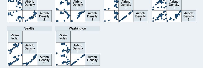
descriptive statistics as well as their corresponding definitions and sources. Figure 1 shows the
correlation coefficients among the three key variables: ZRI (Zillow Index), Airbnb1 (Airbnb Density 1),
and Airbnb2 (Airbnb Density 2). A positive relationship is identified in most of the cities.J. Risk Financial Manag. 2020, 13, 161 8 of 18
Table 1. Neighbourhood characteristics.
Neighbourhood Neighbourhood
City City Size City Population Neighbourhood Neighbourhood
Neighbourhood Population Median Family
Population (km2 ) Density per km2 Population Size (km2 )
Density per km2 Income ($)
Fenway, Boston 695,926 232.1 2998.3886 25,619 3.212 7976.027397 76,643
Logan Square, Chicago 2,705,988 606.1 4464.59 87,509 8.37 10,455.07766 68,223
Venice, LA 10,105,518 1302 7761.5346 27,525 8 3440.625 115,967
Greenpoint, NYC 8,398,748 783.8 10,715.422 36,492 7.133 5115.939997 78,287
Rittenhouse Square, Philadelphia 1,584,138 367 4316.4523 24,219 4.43 5467.042889 138,611
Northwest, Portland 652,573 375.5 1737.8775 17,585 3.44 5111.918605 118,404
La Jolla, San Diego 3,343,364 964.5 3466.422 39,742 23.13 1718.20147 107,094
North Beach, San Francisco 883,305 121.4 7275.9885 26,527 1.27 20,887.40157 66,422
Broadway, Seattle 744,949 217 3432.9447 25,448 4.248 5990.583804 83,403
Georgetown, Washington DC 633,427 177 3578.6836 27,562 3.035 9081.383855 220,000
Table 2. Identification and definition of variables.
Variable Type Variables Description Source
Dependent Variable ZRI A monthly dollar-valued index of the typical market rent at the neighbourhood level Zillow
Airbnb1 Airbnb density as a proportion of the total stock of housing at the neighbourhood level Tom Slee/ACS
Airbnb2 Airbnb density as a proportion of the vacant stock of housing at the neighbourhood level Tom Slee/ACS
Number of listings in City Total number of Airbnb listings at the city-wide level ACS
Total housing stock Estimated number of housing units at the neighbourhood level ACS
Independent Variables Total vacant housing Estimated number of vacant housing units at the neighbourhood level ACS
The number of people unemployed as a percentage of all people aged 16–64 at the
Unemployment rate ACS
neighbourhood level
Median salary The median family income in USD at the neighbourhood level ACS
The number of people with a bachelor’s degree or higher as a percentage of all people aged
% of workforce with bachelors or higher ACS
25–64 at the neighbourhood level
The number of people under the national poverty line as a percentage of all people aged
Poverty level ACS
16–64 at the neighbourhood level
Note: Data sources: Zillow: https://www.zillow.com. Tom Slee: http://tomslee.net. ACS: American Community Survey, https://www.census.gov/programs-surveys/acs.J. Risk Financial Manag. 2020, 13, x FOR PEER REVIEW 9 of 18
J. Risk Financial Manag. 2020, 13, 161 9 of 18
Table 3. Descriptive statistics.
Table 3. Descriptive statistics.
Variables Mean Standard Deviation Minimum Maximum
Variables ZRI Mean3476 Standard 1368
Deviation 1800
Minimum 6030
Maximum
Airbnb1 3.56% 3.27% 0.27% 14.99%
ZRI 3476 1368 1800 6030
Airbnb2
Airbnb1 37.67%
3.56% 32.15%
3.27% 2.48%
0.27% 128.89%
14.99%
Number of listings in City
Airbnb2 37.67%10,801 10,478
32.15% 1275
2.48% 41,245
128.89%
NumberTotal housing
of listings stock
in City 10,80119,515 11,055
10,478 8360
1275 72,330
41,245
TotalTotal vacant
housing housing
stock 19,5152049 1121
11,055 648
8360 6054
72,330
Total Unemployment
vacant housing rate 20496.14% 2.76%
1121 2.11%
648 14.50%
6054
Unemployment
Median salaryrate ($) 6.14%
100,676 2.76%
46,815 2.11%
51,675 14.50%
227,424
Median salary
% of workforce ($)
with bachelor’s or higher 100,676
65.41% 46,815
15.58% 51,675
31.42% 227,424
88.05%
% of workforce with bachelor’s
Poverty levelor higher 65.41%
13.25% 15.58%
7.91% 31.42%
4.17% 88.05%
37.80%
Poverty level 13.25% 7.91% 4.17% 37.80%
Figure
Figure 1. Correlation
1. Correlation betweenproperty
between propertyprice
price index
index and
andAirbnb
Airbnbdensity
densityin ten American
in ten cities.
American cities.
3.4. 3.4. Models
Models
ThisThis paper
paper aimsaims
to to estimateAirbnb’s
estimate Airbnb’simpact
impact onon rents
rentsatataaneighbourhood
neighbourhood level. TheThe
level. hypothesis
hypothesisis is
that higher Airbnb densities in a neighbourhood will increase the rent level due to landlords shifting
that higher Airbnb densities in a neighbourhood will increase the rent level due to landlords shifting
away from supplying the long-term market in favour of the newly available, and more profitable, short-
away from supplying the long-term market in favour of the newly available, and more profitable,
term market. We tested the existence of a long-term relationship between Airbnb densities and rents
short-term
by usingmarket. We regression
panel data tested the method,
existence of the
and a long-term
short-termrelationship between
dynamics between Airbnb
Airbnb densities
densities and and
rentsrents
by using panel data regression method, and the short-term dynamics between Airbnb
by using first differenced linear regression models created with a stepwise selection procedure. densities
and rentsOur
by using first
monthly differenced
data linear regression
cover ten American models
cities over created
the period with a2013
between stepwise
and 2017selection procedure.
1. This gave us
Our
an monthly panel
unbalanced data cover ten
data set of American cities over
254 observations due tothe period
some between
missing values2013 and
at the 20171 . This
beginning of thegave
us an unbalanced panel data set of 254 observations due to some missing values at the beginning of
1 Our sample
the sampling period.period
Westops at 2017 abecause
performed the key
Hausman testAirbnb density
to check information
whether a fixedis effect
unavailable after 2017.
or a random effect
Specifically, Tom Slee stopped releasing such data at his website after 2017.
panel model should be estimated. The test results suggest a random effect model. We estimated the
following two models accordingly
1 Our sample period stops at 2017 because the key Airbnb density information is unavailable after 2017. Specifically, Tom Slee
stopped releasing such data at his website after 2017.J. Risk Financial Manag. 2020, 13, 161 10 of 18
k
X
Yi,t = α + β1 Airbnb1i,t + α j x j,i,t + τi + θi,t (1)
j=1
k
X
Yi,t = α + β1 Airbnb2i,t + α j x j,i,t + τi + θi,t , (2)
j=1
where Yi,t is the ZRI in neighbourhood i at month t; Airbnb1i,t is the measure of Airbnb density
as a proportion of the total stock of housing in the same neighbourhood, i, at month t; Airbnb2i,t
is the measure of Airbnb density as a proportion of the vacant stock of housing; x j,i,t is the jth
neighbourhood-level characteristics in neighbourhood i at month t. τi and θi,t are the within-entity
and between-entity random errors, respectively.
The next step in our empirical investigation was to analyse the response of residential rents to
short-term changes in Airbnb densities. We believe that it is necessary to analyse each neighbourhood
separately through the use of multiple time-series datasets, because Airbnb penetration is likely to
have heterogenous short-term impacts across different cities and neighbourhoods depending on their
locational and demographic characteristics. Unit root tests were performed to check the stationarity of
all variables both at the level and at the first difference. The results are reported in Table 4. Although
most of the variables are not I(0), all of them are I(1), which means estimating first differenced models
by using the OLS regression method will not lead to spurious regression problems. These first
differenced models can ‘help stabilise the mean of a time series by removing changes in the level
of a time series, therefore eliminating (or reducing) trend’ (Hyndman and Athanasopoulos 2018).
Additionally, the first difference approach offers many other benefits. Firstly, according to Wooldridge
(2018), if homoscedasticity is assumed, using a first differenced model will result in a more efficient
estimate of the coefficients when compared to a fixed effects model, the most common alternative.
As will be discussed in further detail, the assumption of serially uncorrelated error terms holds in this
model. Additionally, the procedure can remove or reduce the presence of autocorrelation, whereby the
residuals of the model are not independent from one another, often caused by a common exogenous
element being present in a given time period. First differencing removes this correlation by removing
the fixed effects, or time invariant portion of the error terms
k
X
∆Yi,t = α + β1 ∆Airbnb1i,t + α j ∆x j,i,t + εi (3)
j=1
k
X
∆Yi,t = α + β1 ∆Airbnb2i,t + α j ∆x j,i,t + εi , (4)
j=1
where ∆Yi,t is the first differenced ZRI in neighbourhood i at month t; ∆Airbnb1i,t , ∆Airbnb2i,t and ∆x j,i,t
are the first difference of Airbnb1i,t , Airbnb2i,t , and x j,i,t , respectively. Rather than regressing the ZRI in
neighbourhood i at month t against the corresponding Airbnb density measures and time-varying
characteristics, the model now regresses the change in ZRI against the change in Airbnb densities
and time-varying characteristics across two consecutive time periods in neighbourhood i. In terms of
interpretation, this model allowed us to quantify the effect that a month to month change in Airbnb
density has on the month to month change in ZRI, as characterised by β1 in both sets of models.
We used a stepwise selection algorithm that creates models which include the relevant Airbnb density
metric and only those first differenced time-varying characteristics that have a significant effect on the
first difference of the ZRI. This procedure allows the first differenced models to exclude independent
variables that have insignificant effects on the changes in the ZRI from month to month and, therefore,
helped the paper to better isolate Airbnb’s short-term impact on rents.J. Risk Financial Manag. 2020, 13, 161 11 of 18
Table 4. Unit Root Test Results (level and first differenced series).
Number of Total Total % of Workforce
Unemployment Median Poverty
City N ZRI Airbnb1 Airbnb2 Listings in Housing Vacant with Bachelors or
Rate Salary ($) Level
City Stock Housing Higher Degrees
Level
Fenway, Boston 18 −1.98 −1.19 −1.49 0.41 −5.70 *** −3.04 ** 0.08 −0.22 0.0001 −7.86 ***
Logan Square,
22 −1.46 −2.02 −1.98 −1.84 −9.54 *** −0.04 −7.99 *** −0.22 −0.58 −6.33 ***
Chicago
Venice, LA 27 −2.01 −1.38 −1.41 −0.40 −3.46 ** −4.90 *** −0.70 0.76 0.26 −5.46 ***
Greenpoint, NYC 24 −1.12 −2.35 −2.45 −1.86 0.29 −10.3 *** −9.56 *** 0.07 −0.06 −1.57
Rittenhousen Square,
19 −1.08 −0.95 −1.26 −1.44 1.77 −3.79 *** −10.17 *** −0.41 −1.36 −6.00 ***
Philadelphia
Northwest, Portland 21 −0.02 −3.74 *** −2.78 * −3.40 ** −5.12 *** −8.09 *** −16.5 *** −0.41 −0.22 −3.88 ***
La Jolla, San Diego 21 −1.57 −2.25 −2.21 −0.97 0.70 −8.11 *** −5.57 *** −1.53 −8.11 *** −5.06 ***
North Beach, San
19 0.12 −4.67 *** −2.29 −5.93 *** 2.14 2.42 −5.62 *** 1.45 1.20 1.61
Francisco
Broadway, Seattle 22 0.14 −1.61 0.50 −1.23 −5.00 *** −1.59 −5.98 *** 1.20 0.38 −6.59 ***
Georgetown,
21 −1.63 −0.70 −0.65 −0.55 −9.69 *** 1.21 −0.13 −0.55 −1.23 1.45
Washington DC
First Differenced
Fenway, Boston 17 −2.60 ** −2.81 ** −2.80 ** −2.56 ** −3.48 *** −64.18 *** −3.42 *** −3.51 *** −3.49 *** −3.53 ***
Logan Square,
21 −2.87 ** −4.36 *** −4.37 *** −4.39 *** −2.67 ** −3.66 *** −2.42 ** −2.24 ** −2.24 ** −2.35 **
Chicago
Venice, LA 26 −2.82 ** −7.94 *** −8.03 *** −7.15 *** −3.36 *** −2.48 ** −3.40 *** −2.85 ** −3.32 *** −9.37 ***
Greenpoint, NYC 23 −2.46 ** −4.29 *** −3.64 *** −4.44 *** −2.29 ** −3.68 *** −3.40 *** −2.67 ** −2.13 ** −2.73 **
Rittenhousen Square,
18 −2.23 ** −5.14 *** −5.57 *** −4.71 *** −2.48 ** −52.57 *** −2.66 ** −2.47 ** −2.48 ** −2.73 **
Philadelphia
Northwest, Portland 20 −7.02 *** −7.37 *** −5.90 *** −6.62 *** −2.52 ** −2.68 ** −13.84 *** −2.53 ** −2.52 ** −3.26 ***
La Jolla, San Diego 20 −2.68 ** −5.07 *** −5.20 *** −3.51 *** −2.72 ** −2.77 ** −4.22 *** −2.66 ** −2.72 ** −2.77 **
North Beach, San
18 −3.16 *** −4.37 *** −4.30 *** −3.06 *** −2.92 ** −3.47 *** −3.46 *** −2.60 ** −3.18 *** −2.88 **
Francisco
Broadway, Seattle 21 −1.95 ** −5.33 *** −4.37 *** −3.74 *** −2.24 ** −3.46 *** −3.21 *** −2.74 ** −2.15 ** −2.39 **
Georgetown,
20 −2.15 ** −3.23 *** −3.22 *** −3.13 *** −3.78 *** −4.13 *** −3.18 *** −3.62 *** −2.77 ** −2.76 **
Washington DC
Note: *** p < 0.01; ** p < 0.05; * p < 0.10.J. Risk Financial Manag. 2020, 13, 161 12 of 18
4. Results and Discussion
The results of panel regression are given in Table 5. We found that both Airbnb densities have
a significant and positive impact on the Zillow rent index. In the long run, an increase in Airbnb
density causes local rents to increase too. Although the statistical significance of control variables varies
between the two models, their coefficient estimates have the same sign. Specifically, employment rate
and median salary have significant negative impacts on Zillow rent index in both models; the negative
effect of total housing stock and the positive relationship between poverty level and residential rents
are statistically significant in Model (2) only; the positive effect from number of listings in city and the
percentage of workforce with higher education is significant in Model (1) only. Fisher-type panel unit
root tests based on augmented Dickey-Fuller test were performed on the residuals of both models.
Four methods proposed by Choi (2001) were used in the tests, all of which strongly reject the null
hypothesis that all the panels contain unit roots. We concluded that higher Airbnb densities cause the
neighbourhoods’ rent levels to increase in the long run.
Table 5. Random Effects Panel Regression Results.
Model (1) Model (2)
Intercept 5051.9111 *** 6193.6094 ***
Airbnb1 6023.9382 ***
Airbnb2 627.6814 ***
Number of listings in City 0.0130 ** 0.0102
Total housing stock −0.0579 −0.1300 **
Total vacant housing 0.0846 0.2821 ***
Unemployment rate −7121.2346 *** −9121.1506 ***
Median salary ($) −0.0211 *** −0.0180 ***
% of workforce with bachelors or higher degrees 1861.3594 *** 1037.3335
Poverty level 1476.1232 2274.8055 **
Hausman χ2 (p-value) 0.42 (0.9808) 1.06 (0.9003)
Panel Unit Root Test
(Fisher-type augmented Dickey-Fuller test)
Inverse χ2 (p-value) 44.7605 (0.0012) 44.2980 (0.0014)
Inverse normal (p-value) −3.2211 (0.0006) −3.0816 (0.0010)
Inverse logit (p-value) −3.2948 (0.0009) 3.2055 (0.0011)
Inverse χ2 (p-value) 3.9150 (J. Risk Financial Manag. 2020, 13, 161 13 of 18
Table 6. Results using Airbnb density as a proportion of the total supply of housing.
Rittenhousen Georgetown,
Fenway, Logan Square, Greenpoint, Northwest, La Jolla, San North Beach, Broadway,
City Venice, LA Square, Washington
Boston Chicago NYC Portland Diego San Francisco Seattle
Philadelphia DC
Intercept 3.24 −13.05 ** 40.72 * −1.74 8.04 −45,871.96 * 142.22 *** −1707.19 *** 3.74 9.35
Airbnb1 4460.19 ** 31,299.19 *** 7.71 −719.5 −1419.54 3160.86 3005.62 58,812.12 *** 4899.93 −6743.13
Number of listings in City −0.05 *** −0.13 **
Total housing stock 1492.42 * 20.00 **
Total vacant housing −0.45 * −84.02 *** 13.7 ***
Unemployment rate 3277.58 −12,370.93 *** −8,426,990.24 * 141,876.29 *** −1,253,372.6 ***
Median salary −0.04 **
% of workforce with
8,009,357.74 * 628,373.09 ***
bachelor’s or higher
Poverty level 2967.97 ** 9172.82 *** −385,971.61 ***
R2 0.35 0.66 0.16 0.14 0.32 0.82 0.90 0.75 0.08 0.02
Adjusted R2 0.28 0.61 0.09 0.08 0.24 0.76 0.88 0.69 0.03 −0.03
Note: *** p < 0.01, ** p < 0.05, and * p < 0.1.
Table 7. Results using Airbnb density as a proportion of the vacant supply of housing.
Rittenhousen Georgetown,
Fenway, Logan Square, Greenpoint, Northwest, La Jolla, San North Beach, Broadway,
City Venice, LA Square, Washington
Boston Chicago NYC Portland Diego San Francisco Seattle
Philadelphia DC
Intercept 3.5 −14.3 ** 40.64 * −1.31 8.00 −45,485.37 * 142.67 *** −1602.4 *** 2.43 9.45
Airbnb2 590.42 ** 3407.88 *** 6.2 −61.39 −189.13 263.89 425.98 7601.54 *** 296.07 * −702.68
Number of listings in City −0.05 *** −0.15 ***
Total housing stock 1479.37 * 18.53 **
Total vacant housing −0.46 * −84.15 *** 13.76 ***
Unemployment rate −12,675.23 *** −8,348,757.25 * 142,468.8 *** −1,183,308.56 ***
Median salary −0.04 **
% of workforce with
7,945,874.66 * 593,580.91 ***
bachelor’s or higher
Poverty level 3116.31 ** 9267.79 *** −387,672.23 ***
R2 0.27 0.66 0.16 0.14 0.32 0.82 0.90 0.77 0.17 0.02
Adjusted R2 0.24 0.61 0.09 0.08 0.25 0.76 0.88 0.71 0.12 −0.03
Note: *** pJ. Risk Financial Manag. 2020, 13, 161 14 of 18
Additionally, when examining Airbnb density as a proportion of a neighbourhood’s vacant
supply of housing, four of the ten neighbourhoods show a significant positive relationship between
Airbnb usage and rents. These results are consistent with both the supply side theory mentioned
previously and Airbnb’s hypothesised stock reallocation effects. More specifically, the home-sharing
premium results in an increased number of Airbnb units available relative to the number of vacant
dwellings, which puts upward pressure on rents due to the fact that some of the supply of long-term
accommodation has been reallocated to the short-term market.
This being said, however, the relationship is far from unanimous. Consistent with the findings of
Garcia-López et al. (2019), the large variance in values of Airbnb density coefficients indicates that
home-sharing has had heterogenous effects on neighbourhoods’ rental markets. Using the first density
metric, the models indicate that a one-unit monthly increase in Airbnb density rates can increase
the ZRI by anywhere between 7.71 dollars, in the case of Venice, and 58,812 dollars, in the case of
North Beach. The variance is similar when using the density measure as a proportion of vacant stock,
as coefficients range from 6.2 dollars in Venice to 7601 dollars in North Beach. Whilst the upper end
of this spectrum is suspiciously high, it is important to note that at the end of the research period,
North Beach had a density measure of just 0.94%. Therefore, whilst an increase of $7601 is high, a one
percentage point increase in Airbnb density could indeed have a large effect on the rental index in
the neighbourhood.
Additionally, when examining the maturity of the Airbnb markets in these neighbourhoods,
an obvious pattern emerges. As expected, the neighbourhoods with the highest Airbnb density rates
at the end of the research period are also those where β1 is the lowest, in absolute terms. That is,
when Airbnb units already account for a large proportion of the total and vacant stock of housing,
a one-unit monthly increase in the Airbnb density measures will change the ZRI the least, both
positively and negatively.
Interestingly, the neighbourhoods that exhibit a significant positive relationship between Airbnb
density rates and rents are also those with some of the highest population densities; this being Fenway,
Logan Square, and North Beach. This relationship may be due to the fact that the housing markets in
these neighbourhoods are already saturated and under strain. However, due to the small sample size
of neighbourhoods analysed, it is difficult to comment on the broader relationship between population
densities and the impact that Airbnb has on rental markets.
In terms of the time-varying characteristics included in our models, it becomes apparent that few
affect the level of rents in a consistent manner. As can be seen from both tables, the use of the stepwise
selection procedure has meant that some neighbourhoods’ models include many more time-varying
characteristics than others. Additionally, many of the variables that were included have inconsistent
signs, contradicting previous research and perhaps underlining one limitation of the first differenced
models. Furthermore, the models’ ability to explain the variation in monthly changes in the ZRI differ
dramatically: in some neighbourhoods, the first differenced model explains 90% of the variation in
ZRI values, as can be seen from La Jolla, whilst in others, such as Broadway, it explains just 8%. Thus,
whilst in some neighbourhoods these first differenced models are relatively successful in estimating
ZRI levels, they are far from being a perfect predictor.
5. Policy Implications
Despite the recent scholarly investigations into Airbnb’s effects on rental markets, policy makers
tasked with regulating the unprecedented growth of home-sharing platforms have had inadequate
information with which to make effective ‘informed’ policy decisions (Horn and Merante 2017). Rather
than using evidence-backed approaches, they have often relied on the recommendations of academics
in order to ‘curb Airbnb’s impacts on a neighbourhood’s character and housing while harnessing the
economic activity it brings’ (Lee 2016, p. 229). This has led to attempts at regulation across cities
differing in both approaches and aims. On one end of the spectrum, policymakers have looked to
engage in the free market ‘laissez-faire’ approach whereby they have not engaged in regulation orJ. Risk Financial Manag. 2020, 13, 161 15 of 18
have done so in collaboration with these home-sharing platforms. On the other end are policies that
have used existing planning regulations in order to restrict growth or entirely curb the operation of
the platforms (Ferreri and Sanyal 2018). Examples of attempts at regulation in cities across the world
include: a requirement to have a specific permit (Barcelona, Berlin, Paris, and San Francisco), paying
an increased rental tax (Amsterdam and San Francisco), and outlawing STRs or restricting the number
of days that they can be in operation (Berlin, New York, and Amsterdam) (Garcia-López et al. 2019).
It is also important to note that the vast majority of policies implemented by governments in the past
have been backwards looking; that is, they have looked to mend the negative effects that Airbnb has
had on their rental markets rather than curb its future impact.
In order to lessen the negative impact Airbnb has on housing whilst still harnessing its economic
potential, a policy recommendation must take into account several factors. Firstly, as examined earlier,
Airbnb’s heterogenous effect at the neighbourhood level means that no single policy measure can be
implemented to address the effects associated with the home-sharing platform. Rather, each policy
recommendation must be tailored specifically to a district or neighbourhood. Secondly, whilst it is
tempting for governments to create policy measures that look to treat Airbnb’s past impacts, it is likely
that these effects will change as the platform matures and therefore makes it important to forecast
future impacts. Finally, whilst home-sharing platforms often exacerbate the affordability issues present
in many neighbourhoods, it is important that governments look to solve the root cause of this problem
if they want to help their local residents by facilitating the creation of a more equitable housing market
in the future.
In response to the positive correlation between Airbnb penetration and rents, policy makers and
academics have often suggested a blanket ban on home-sharing platforms and STRs. With this in
mind, Koster et al. (2018) attempted to assess the effectiveness of Home Sharing Ordinances (HSOs),
a type of ban, in Los Angeles’ housing market. More specifically, the researchers analysed the change
in Airbnb penetration as well as rental rates in areas close to the borders of cities that had implemented
the HSOs. In effect, they replicated a controlled experiment in order to quantify the policy’s effects.
They found that HSOs were indeed effective at reducing the number of Airbnb listings, with the policy
lowering the number of ‘entire flat’ listings by almost 50% in the long run. Additionally, in using a
differences-in-differences estimation, they were able to show that, on average, the HSOs were able to
reduce rents in the cities by 2%. This being said, however, this type of policy has little impact on the
larger issue. This is evidenced by Lee (2016), who used qualitative interviews as well as economic
theory to argue that, whilst a blanket ban on STRs would remove Airbnb’s role in Los Angeles’
affordability crisis, it would also deprive the city of the economic benefits associated with STRs and
would not help increase the stock of affordable housing.
Instead of an outright ban, a more appropriate measure could be a system of taxation that solely
targets commercial operators. This would enable local governments to generate revenues, in the
form of occupancy tax, from the incomes earned by commercial operators, who are often accused of
knowingly evading taxes through the use of these home-sharing platforms. Not only would the policy
deter the commercial use of Airbnb whilst still allowing local landlords to rent out their excess space,
but the tax revenue generated could help fund the development of additional affordable housing units
and target the larger problem at hand.
Furthermore, policy makers should consider using geographically targeted restrictions which
would only allow Airbnb STRs in buildings that meet a target affordability threshold, as proposed by
Lee (2016). Theoretically, this policy should incentivise large commercial operators to subsidise rents
in some of their units so that they are able to rent out others in the short-term market and tap into
the home-sharing premium. Additionally, Lee (2016) also argues for the use of Community Benefit
Agreements (CBAs), which are contracts that allow for the use of Airbnb if certain conditions are met,
usually to do with the creation, or the setting aside, of affordable housing units. He argues that this
would remove pressure on rents due to Airbnb, allow cities to benefit from the economic efficiencies of
short-term renting, and simultaneously increase the stock of affordable housing (Lee 2016).You can also read