The structure of first cousin marriages in Brazil - Nature
←
→
Page content transcription
If your browser does not render page correctly, please read the page content below
www.nature.com/scientificreports
OPEN The structure of first‑cousin
marriages in Brazil
Paulo A. Otto1, Renan B. Lemes1, Allysson A. Farias1, Mathias Weller2, Shirley O. A. Lima2,
Victor Alves Albino2, Yanna K. Marques‑Alves2, Eliete Pardono1, Magnolia A. P. Bocangel1 &
Silvana Santos2*
This paper deals with the frequency and structure of first-cousin marriages, by far the most important
and frequent type of consanguineous mating in human populations. Based on the analysis of large
amounts of data from the world literature and from large Brazilian samples recently collected,
we suggest some explanations for the asymmetry of sexes among the parental sibs of first-cousin
marriages. We suggest also a simple manner to correct the method that uses population surnames
to assess the different Wright fixation indexes FIS, FST and FIT taking into account not only alternative
methods of surname transmission, but also the asymmetries that are almost always observed in the
distribution of sexes among the parental sibs of first-cousins.
The structure of first-cousin marriages has been the subject of several investigations starting some 60 years ago,
with at least three of them performed in B razil1–3. The first-cousin marriages can be classified into four subtypes,
according to the gender of the two sibs parents of the couple of cousins, as shown in Fig. 1: in subtype A, the
couple of first cousins are the offspring of two sisters; in subtype B, the mother of the male cousin is the sister
of the father of the female cousin; subtype C is the inverse of subtype B; finally, in subtype D, the couple of first
cousins are the offspring of two brothers. In some papers the subtypes A, B, C, and D are alternatively named
3, 4, 2, and 1, respectively. Subtypes A and B, for allowing occasionally the formation of X-linked autozygous
daughters from the couple of first cousins, are also known in the literature by the name X-inbred, while subtypes
C and D, for blocking the formation of autozygous female offspring, receive the name of X-outbred. It is interest-
ing to note that almost always the observed relative frequencies of subtypes A, B, C, and D differ significantly
from equal (1/4) expected population frequencies.
The population average probability of homozygosity by descent (autozygosity) is commonly estimated from
the analysis of sets of genealogies and quantified by Wright’s fixation index FIT. This index takes into account not
only cases of panmixia deviations measured by the fixation index FIS but also cases in which the homozygosity
is due to small population size and other random effects (quantified by the fixation index FST). Because an indi-
vidual cannot be homozygous due to both inbreeding and random effects, F IT is not obtained by simply adding
FIS and FST: the intersection F
IS. FST should be subtracted from this sum. The same result is obtained from the
equation (1 − FIT) = (1 − FIS).(1 − FST).
The probability of a male or female conceptus being homozygous by descent as to the alleles from any
autosomal locus is the inbreeding coefficient F = 1/16, independently from the structure A, B, C, or D of the
first-cousin marriage. The deleterious effects of pathological autosomal recessive alleles (occasionally carried in
more than 1,000 different loci) has been easily demonstrated not only through empirical studies (that compare
morbidity and mortality rates in the offspring of unrelated and consanguineous couples) but also by predictive
theoretical models as well4.
The probabilities of a female concept being homozygous by descent as to alleles carried by an X-linked locus
in subtypes A, B, C, and D are, respectively, F A = 2(1/2)5 + (1/2)3 = 3/16, FB = 2(1/2)4 = 1/8, FC = 0, and FD = 0; if
the four subtypes occur in the population with approximately equal (1/4) frequencies, the average value of the
inbreeding coefficient becomes F = 5/64 = 0.0781. The additional deleterious effect due to this should be not only
modest but also very difficult to estimate because (1) the genes on the X chromosome represent just about five
percent of all genes contained on the human genome; and (2) the deleterious alleles in the X loci are submitted
1
Departamento de Genética e Biologia Evolutiva, Instituto de Biociências, Universidade de São Paulo, Rua do
Matão 277, São Paulo, SP 05508‑090, Brazil. 2Núcleo de Estudos em Genética e Educação, Universidade Estadual
da Paraíba, Rua das Baraúnas, s/n ‑ Prédio da Integração Acadêmica ‑ sala 329, Campus I – Bodocongó, Campina
Grande, Paraíba, Brazil. *email: silvanaipe@gmail.com
Scientific Reports | (2020) 10:15573 | https://doi.org/10.1038/s41598-020-72366-z 1
Vol.:(0123456789)www.nature.com/scientificreports/
Figure 1. Subtypes of first-cousin marriages (see text for details).
to a selection process much stronger than the corresponding one to autosomes, because they are in hemizygous
state among male individuals, and therefore with a much smaller frequency than their autosomal c ounterparts5.
Crow and M ange6 introduced a method that uses the frequencies of population surnames and marriages of
persons with the same surname to estimate the different fixation indexes F IT, FIS and F
ST. The original method
can be applied only to literate populations with a fixed manner of surname transmission and with no asymmetry
in types A, B, C, and D. The method was revisited by several authors, including Cabello and Krieger7, who made
room in it for the asymmetry of patrilineal subtype D.
The first (and main) objective of the present paper is to provide explanation on the frequency asymmetry of
types A, B, C, and D, a topic still not solved in a completely satisfactory manner in the literature.
The second objective of this work is to adapt the isonomy method taking into account not only distortions in
the frequencies of types A, B, C, and D but also the variable mode of surname transmission in poorly accultur-
ated populations without fixed rules.
Results
Asymmetry of first‑cousin subtypes A, B, C, and D. With the aim of obtaining a global vision of the
distribution of subtypes A, B, C, and D, we reduced drastically the number of population samples shown in
Tables IS to IVS of supplementary material, agglomerating all regional groups shown to be homogeneous after
the application of standard chi-squared heterogeneity tests (results detailed on supplementary Table VS). The
various samples from four countries resisted to this process of coalescence (Israel; Japan; Jordan; and Spain).
The 18 groups from Japan could be coalesced in only two subpopulations, rural (14 groups) and urban (four
groups). In the case of Spain, two groups (B-C) out of the four could be considered as one population. With the
application of this procedure, the total of 126 different individual samples listed in Tables IS to IVS (supplemen-
tary material) reduced to just 28, as shown in Table 1, which summarizes the results of descriptive analysis from
these new results.
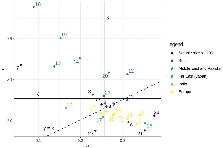
All data from Table 1 are plotted in the graph of Fig. 2, in which the abscissae axis (x) corresponds to the
values of a = A/N and the ordinates axis (y) to the values of d = D/N. The graph shows also the straight lines
that represent the average values of a and d estimated from all populations shown, as well as the line a = d. The
plotted circles in purple correspond to samples with small sample sizes (less than 100): 6 Chile, 20 (Korea), 21
(Norway), 26 (Sweden) and 27 (United States). These numbers, as well all others shown in Fig. 2, correspond to
the leftmost figures identifying the population samples listed on Table 1.
The influence of ruralization and urbanization and of other factors such as different mobility rates among
males and females on the frequency of first-cousin marriage subtypes A, B, C, and D has been discussed in the
literature1,8, however without any results that can be generalized, probably due to temporal, geographical and
cultural differences in relation to the concepts of what is rural or urban in different populations. For example,
a community considered as rural in present Belgium probably corresponds to urban life in a large city fairly
developed in a poorly developed and industrialized country, in which an area categorized as rural in present times
surely corresponds to a rural area in fully developed and industrialized countries many decades ago. Taking this
reasoning into account, the agglomeration of rural or urban areas from geo-politically distinct regions makes no
sense at all. The Japanese reports (as well as other researches developed in Japan by American geneticists), on the
other hand, have an astonishing amount of reliable information as to the rural or urban character of the samples,
but their data were used generally with the main aim of comparing the viability, morbidity, and mortality of the
offspring in subtypes A, B, C, and D. The heterogeneity test in 14 samples collected in rural areas (Hirado A,
Hoshino, Ina, Kurogi, Kyushu, Mishima, Nansei, Nanto, Okayama, Onodani, Oshima, Shizuoka A, Shizuoka B,
Shizuoka C) showed that they could be coalesced, the same occurring with four urban localities (Fukuoka, Hirado
B, Hiroshima A, Hiroshima B) (Table VS). Testing the hypothesis that the distribution of subtypes A, B, C, and
D is aleatory (expected frequency of each class = 1/4) in the urban and rural samples resulting from four and 14
subsamples respectively, we found that the observed frequencies are significantly different from the expected by
chance (p-value < 0.0001). By comparing both coalesced samples through a chi-squared test on a contingency
table, a very significant chi-squared value (p-value < 0.0001) was obtained; the analysis of the adjusted residuals
(Pearson/Haberman test) showed that there is a significant increase of subtype A and a significant decrease of
the other subtypes (B, C, and D) in the urban communities and the opposite in rural ones.
Scientific Reports | (2020) 10:15573 | https://doi.org/10.1038/s41598-020-72366-z 2
Vol:.(1234567890)www.nature.com/scientificreports/
Sample Locality N a = A/N b = B/N c = C/N d = D/N a+b c+d %fem %mal F
1 Austria 822 0.33333 0.27981 0.20560 0.18127 0.61314 0.38687 0.57604 0.42398 0.09748
2 Belgium 210 0.23333 0.26667 0.23333 0.26667 0.50000 0.50000 0.48333 0.51667 0.07708
3 Brazil NE old 1809 0.22886 0.24433 0.20122 0.32559 0.47319 0.52681 0.45164 0.54836 0.07345
4 Brazil SE old 1,036 0.26158 0.24807 0.22297 0.26737 0.50965 0.49034 0.49710 0.50289 0.08006
5 Brazil NE new 909 0.27063 0.20462 0.26183 0.26293 0.47525 0.52476 0.50385 0.49616 0.07632
6 Brazil SE new 989 0.31345 0.28514 0.21234 0.18908 0.59859 0.40142 0.56219 0.43782 0.09441
7 Chile 17 0.05882 0.35294 0.11765 0.47059 0.41176 0.58824 0.29412 0.70588 0.05515
8 England 296 0.34122 0.22973 0.20608 0.22297 0.57095 0.42905 0.55912 0.44088 0.09270
9 Germany 1617 0.29314 0.27149 0.21831 0.21707 0.56463 0.43538 0.53804 0.46197 0.08890
10 India 290 0.16552 0.30000 0.27586 0.25862 0.46552 0.53448 0.45345 0.54655 0.06854
11 Israel A 598 0.31104 0.21405 0.17726 0.29766 0.52509 0.47492 0.50670 0.49331 0.08508
12 Israel B 212 0.31132 0.16981 0.09434 0.42453 0.48113 0.51887 0.44340 0.55660 0.07960
13 Israel C 456 0.13816 0.24561 0.15351 0.46272 0.38377 0.61623 0.33772 0.66228 0.05661
14 Israel D 509 0.19843 0.15324 0.14538 0.50295 0.35167 0.64833 0.34774 0.65226 0.05636
15 Italy 4,384 0.27714 0.29037 0.20963 0.22286 0.56751 0.43249 0.52714 0.47286 0.08826
16 Japan URB 2,263 0.35307 0.26646 0.19620 0.18427 0.61953 0.38047 0.58440 0.41560 0.09951
17 Japan RUR 1648 0.25364 0.30825 0.22209 0.21602 0.56189 0.43811 0.51881 0.48119 0.08609
18 Jordan A 303 0.08911 0.09901 0.05611 0.75578 0.18812 0.81189 0.16667 0.83334 0.02908
19 Jordan B 360 0.15278 0.16667 0.07778 0.60278 0.31945 0.68056 0.27500 0.72500 0.04948
20 Jordan C 487 0.26694 0.18480 0.11499 0.43326 0.45174 0.54825 0.41684 0.58316 0.07315
21 Korea 54 0.35185 0.37037 0.12963 0.14815 0.72222 0.27778 0.60185 0.39815 0.11227
22 Norway 112 0.25000 0.22321 0.25000 0.27679 0.47321 0.52679 0.48660 0.51340 0.07478
23 Pakistan 516 0.25581 0.25194 0.17442 0.31783 0.50775 0.49225 0.46899 0.53101 0.07946
24 Spain A 3,160 0.31171 0.27152 0.21076 0.20601 0.58323 0.41677 0.55285 0.44715 0.09239
25 Spain B + C 1652 0.27966 0.27482 0.21489 0.23063 0.55448 0.44552 0.52452 0.47549 0.08679
26 Spain D 3,250 0.26185 0.27815 0.21846 0.24154 0.54000 0.46000 0.51016 0.48984 0.08387
27 Sweden 34 0.23529 0.44118 0.17647 0.14706 0.67647 0.32353 0.54412 0.45589 0.09926
28 United States 104 0.37500 0.19231 0.21154 0.22115 0.56731 0.43269 0.57692 0.42308 0.09435
Table 1. Descriptive analysis of the results obtained after agglutinating all geographically similar subsamples
shown in Tables IS to IVS (supplementary material): (1) Austria, (2) Belgium (two agglutinated subsamples),
(3) NE Brazil (Freire-Maia; four agglutinated subsamples), (4) S/SE Brazil (Freire-Maia; seven agglutinated
subsamples), (5) NE Brasil (Paraíba; 35 agglutinated subsamples), (6) SE Brazil (Laboratório de Genética
Humana USP; 32 agglutinated subsamples), (7) Chile, (8) England (three agglutinated subsamples), (9)
Germany (three agglutinated subsamples), (10) India (three agglutinated subsamples), (11–14) Israel A,
B, C and D, (15) Italy, (16) Japan (four agglutinated urban subsamples), (17) Japan (14 agglutinated rural
subsamples), (18–20) Jordan A, B and C, (21) Korea, (22) Norway, (23) Pakistan, (24) Spain A, (25) Spain
B + C (two agglutinated subsamples), (26) Spain D, (27) Sweden, (28) United States. N : sample size (number
of first cousin couples); a, b, c, d, a + b, c + d : frequencies of subtypes A, B, C, D, A + B e C + D; %fem e %mal:
percentages of women and men among the parental sibs of the first cousins; F: average inbreeding coefficient of
the feminine offspring, taking into account the observed frequencies a, b, c, and d.
Since the use of variables d = D/N and a = A/N, respectively on ordinates (y) and abscissas (x) axes in Fig. 2
seem to be sufficient for causing a reasonably good dispersion in the set of plotted data, we present in detail,
on Fig. 3, the results corresponding just to the samples collected in Brazil. The individual values of the samples
are represented by clear dots, with the exclusion of all subsamples with size less than 20. With this strategy the
number of samples collected in the state of Paraiba in NE Brazil reduced from 35 to 17. The filled symbols n1,
n2, s1, and s2 correspond to the average values of a and d in the samples of N E1,2, NE (present work), S/SE1,2,
and SE (present work) regions. The graph shows also the average values of a and d for the NE and SE regions,
that are situated exactly in the intersection of the straight lines corresponding to the average allover values of a
and d for these regions.
Figure 3 shows that subtype D frequency value is predominant in the old NE sample while subtype A fre-
quency value is predominant in the new SE sample, the first above the global averages of d for both NE and SE
regions and below the global average of a for both regions; and the second value one below the global averages
of d for both NE and SE regions and above the global average of a for both regions. The values corresponding to
the most recent NE sample and to the old S/SE regions are very similar and exactly intermediary in relation to
the global allover average values of a and b.
Estimate of FIT through the analysis of the pattern of surname transmission in Northeastern
Brazil. The method of Crow and Mange6, briefly described in the lines below for the case of first cousin mar-
Scientific Reports | (2020) 10:15573 | https://doi.org/10.1038/s41598-020-72366-z 3
Vol.:(0123456789)www.nature.com/scientificreports/
Figure 2. Distribution of a = A/N and d = D/N values in the samples described on Table 1, identified by the
figures shown at the leftmost column of this table.
Figure 3. Distribution of a = A/N and d = D/N values in the Brazilian samples (see details and explanations on
the text above).
riages, is based on the existence of: (1) rigid and fixed rules of surname transmission (generally or exclusively
patrilineal or matrilineal); (2) a balanced (random) distribution of subtypes A, B, C, and D; and (3) surnames
that have been generated just once in the population; under this last hypothesis, individuals with the same sur-
name must have some degree of biological relationship.
If the observed population frequency of couples with the same surname is P, the approximate value of F IT
can be obtained from FIT = P/4. If pi and qi are the proportions of men and women with a given surname, the
population expected frequency of couples with this surname will be, on the hypothesis of random mating, piqi,
and its contribution to the inbreeding coefficient will be piqi/4; and the contribution of all surnames to the
random inbreeding coefficient will be F ST = ∑piqi/4. From F IT = FST + FIS − FISFST we obtain the estimate of the
non-random inbreeding coefficient FIS = (FIT − FST)/(1 − FST) = (P − ∑piqi)/(4 − ∑piqi) obtained from the analysis
of surname population frequencies. Under the hypothesis that surnames occur with same frequencies among
males and females ( pi = qi), it comes out that p iqi = pi2; and the above formula can therefore be simplified to
FIS = (P − ∑pi2)/(4 − ∑pi2).
The authors of the method called attention to the problems of its application in poorly acculturated popula-
tions, without fixed rules of surname transmission. In the lines below we adapt the method to the population of
the rural municipality of Brejo dos Santos, in the state of Paraiba in the Brazilian NE region, taking into account
(1) the non-random distribution of sexes among the pairs of parental sibs of the consanguineous couples; and
(2) the irregular mode of surname transmission in the population, that can take place: (1) strictly through the
father; (2) strictly through the mother; (3) with an uncertain mode (case that takes place when both parents
have the same surname that is transmitted to their offspring); and (4) when the offspring has surnames different
from those of both parents.
Scientific Reports | (2020) 10:15573 | https://doi.org/10.1038/s41598-020-72366-z 4
Vol:.(1234567890)www.nature.com/scientificreports/
Mode of surname transmission in the population. The studied sample was composed by 538 individuals with
twice-checked information; in 243 of them the offspring surname was received only from the father, in 112 it was
transmitted only by the mother; in 95 cases the surname didn’t originate from either parent; and in 88 cases the
transmission mode could not be ascertained (parental pair with the same surname). The data from 90 women
that had the marriage surname of their spouses, without reliable information as to their family surname, were
previously excluded from the sample. Assuming that in the 88 cases of couples with the same surname the trans-
mission took place patri- or matrilinearly after the proportions 243 : 112 respectively, we obtain the corrected
proportions of transmission occurring patri- and matrilinearly, respectively, 243(1 + 88/355)/538 = 0.5636 and
112(1 + 88/355)/538 = 0.2598.
Surname distribution in the population and in the couples. In the calculations shown below, we considered 233
marriages that did not contain the 90 women without reliable information as to their family surname. Some
men and some women from this population married twice or more times; this explains the fact that the totals of
men and women that married are smaller than the total number of marriages (233), corresponding respectively
to 219 and 225.
The masculine surnames were the following: Silva (63/219 = 0.288), Oliveira (24/219 = 0.110), Sousa
(17/219 = 0.078), Costa (9/219 = 0.041), Diniz and Lima (8/219 = 0.037), Santos (7/219 = 0.032), Freitas and
Melo (6/219 = 0.027), Bezerra (4/219 = 0.018), Almeida, Barbosa, Barreto, Dantas, Pereira, and Sobrinho
(3/219 = 0.014); all other masculine surnames occurred each in just 1 or 2 individuals, therefore with a frequency
of less than 1%.
The most common feminine surnames were: Silva (52/225 = 0.231), Conceição (23/225 = 0.102), Sousa
(22/225 = 0.098), Freitas (19/225 = 0.084), Oliveira (17/225 = 0.076), Lima (9/225 = 0.040), Diniz (6/225 = 0.027),
Araujo, Costa, Jesus, Sá, and Santos (4/225 = 0.018), Bezerra, Brito, Dantas, Guedes, Melo, and Vieira
(3/225 = 0.013); all other surnames occurred in just 1 or 2 individuals each, therefore with a frequency of less
than 1%.
Considering the total sample of 444 male and female individuals, the surnames that occurred in more than 4
individuals (therefore with a frequency larger than 1%) were: Silva (115/444 = 0.259), Oliveira (41/444 = 0.092),
Sousa (39/444 = 0.088), Freitas (25/444 = 0.056), Conceição (23/444 = 0.052), Lima (17/444 = 0.038), Diniz
(14/444 = 0.032), Costa (13/444 = 0.029), Santos (11/444 = 0.025), Melo (9/444 = 0.020), Bezerra (7/444 = 0.016),
Araújo and Dantas (6/444 = 0.014), Barreto and Sá (5/444 = 0.011).
Estimation of fixation indexes FIT, FST, and FIS. Using the data from Table VIS and applying to them, without any
correction, the formulas proposed by Crow and Mange6, we obtain
P = 39/233 = 0.1674
pi qi = 0.0901
FIT = P/4 = 0.0418
FST = �pi qi /4 = 0.0225
FIS = (FIT − FST )/(1 − FST ) = 0.0197
As shown in Table IS, in the municipality of Brejo dos Santos the frequencies of subtypes A, B, C and D of
first cousin marriages were respectively 0.2169, 0.2530, 0.2048, and 0.3253. Taking into account that in this
locality the frequencies with which the surname is patrilinearly and matrilinearly transmitted are 0.5636 and
0.2598 respectively, a gross correction of the factor 0.25 that occurs in the formulas of Crow and Mange can be
obtained from 0.2169 × 0.2598 + 0.3253 × 0.5636 = 0.2397 ~ 0.24. The estimates of the three fixation indexes FIT,
FST, and FIS then become
FIT = 0.24 × P = 0.0402
FST = 0.24 × pi qi = 0.0216
FIS = (FIT − FST )/(1 − FST ) = 0.0190
Rates of intentional (inbreeding strictly speaking) and random consanguineous matings in NE Brazil. The impor-
tance of the surname method is that it enables the indirect estimation of the factors responsible for the consan-
guineous marriages. Since all figures obtained for the estimates F IT, FST, and F
IS are positive, we can obtain the
approximate proportion of first cousin marriages due to intentional factors (inbreeding), which is 0.47 or about
50%.
Table 2 (adapted from Weller et al.9) shows the estimates of population size, frequency of consanguineous
marriages and the average value of the inbreeding coefficient FIT of a set of rural localities in the state of Paraiba
in NE Brazil. The table originally published contains data from 39 localities, not including the data from Gurjão
and Lagoa Seca (shown in Table IS) and including six localities not shown in the same table (Belém, Cajazerinhas,
Scientific Reports | (2020) 10:15573 | https://doi.org/10.1038/s41598-020-72366-z 5
Vol.:(0123456789)www.nature.com/scientificreports/
Sample n frcc FIT
1 28,299 0.1929 0.00651
2 33,031 0.1623 0.00380
3 55,469 0.1671 0.00509
4 13,821 0.1912 0.00724
5 4,416 0.2049 0.00604
Table 2. Estimated population sizes (n), observed frequencies of consanguineous mating (frcm), and average
fixation index (FIT) in localities from NE Brazil (state of Paraíba). All data were adopted and condensed from
Weller et al.9, taking into account population size intervals of 10,000. (1) Average values of Catolé do Rocha
and Pombal, (2) São Bento; (3) Sousa; (4) Uiraúna; (5) average values of all other localities (including Brejo dos
Santos), each with a population size less than 10,000.
Figure 4. Indication of a negative correlation between the frequency of consanguineous mating and population
sizes in the state of Paraiba in NE Brazil (data taken from Weller et al.9). The black line corresponds to the
regression line of the data.
Matinhas, Poço Dantas, Sousa and Vierópolis). Brejo dos Santos is included in Table 2 among the localities with
a population size of less than 10,000.
Since the surname method indicated a frequency of about 50% of consanguineous marriages taking place due
to intentional factors (strict sense inbreeding), it is expected that an inverse correlation (or at least a tendency)
exists between the population sizes and the frequency of consanguineous mating occurring in them. In order
to verify this point, the data from Table 2 (frcm and n) were submitted to a simple model of linear regression
analysis, after applying to the dependent variable (frcm) the transformation arc-sin(x)1/2 with the aim of nor-
malizing its distribution. The results of this analysis revealed the existence of a tendency, with the values of frcm
being roughly estimated by the formula frcm = 0.2688—0.0056n; r 2 = 0.6675; F(1;3) = 6.021 (p-value = 0.09), as
shown in the graph of Fig. 4.
Discussion and conclusions
Consanguineous marriages still take place at significant proportions worldwide (at least 10% of all human
unions), being a frequent practice not only among Muslim populations (in the Middle East, North Africa, and
West Asia) and in some regions of India but also in many areas (especially rural, isolated, and underdeveloped
ones) throughout the whole w orld10–14. By far the most common type of consanguineous marriage is the first-
cousin one, which accounts generally for proportions as high as 30% to 50% or even more of all mating taking
place between relatives in a given population11,13,14. Although there is currently no general consensus about the
reasons that favor the occurrence of consanguineous mating in such high rates, and probably because of its very
complicated multifaceted nature, the issue has been subjected to a large number of different well-planned stud-
ies, an important list of which is found in www.consang.net14. These studies were able to suggest explaining
factors related to social, religious, cultural, political, and economical status, as well as the smaller size of isolated
rural populations13,15. For example, in Arab populations consanguineous marriages are favoured because unions
between non-relatives are thought to be less stable, since in marital disputes the husband’s family would side
with the consanguineous w ife11,16–18.
An important issue is why particular types of first cousin unions are strongly favored in some major popula-
tions, e.g. patrilineal parallel cousin marriage (type D) in Muslim Arab communities, but prohibited in others19,
a result also observed by us. The scatter diagram of Fig. 2 draws immediate attention to this fact. In more than
Scientific Reports | (2020) 10:15573 | https://doi.org/10.1038/s41598-020-72366-z 6
Vol:.(1234567890)www.nature.com/scientificreports/
half of the samples we selected (numbered as 12, 13, 17, 18, and 22), corresponding to Near and Middle East
populations with more rigid and strict traditional patriarchal rules, the subtype D is larger than A. This tendency
might be explained by the simple fact that in strongly patriarchally rooted populations or communities the father
of the bride or bridegroom, when arranging a consanguineous marriage within his family, will preferentially
choose the partner cousin among the offspring of his brothers in flagrant detriment to the offspring of his sisters.
This tendency is strikingly downplayed in the majority of other population groups, as the graph of Fig. 2
clearly shows. When Southern Indian Hindus are considered, for example, the situation is reversed, because
parallel cousin unions (types A and D) are forbidden in Hindu society20. This simple fact probably explains per
se the lower frequency (of about 40%) of types A and D in the Indian samples (123 out of 290 first-cousin mar-
riages) we included in the present study.
The separate analysis of the four Brazilian samples (Table 1 and Fig. 3) indicates an overwhelmingly predomi-
nant increase of the subtype D in the old NE sample, above the overall average values of D for both geographical
regions NE and SE and far below from the global averages value of A for the same regions. This predominance
is fairly suggestive of a more stringent application of patriarchal rules, a common issue in old rural areas of NE
Brazil; just the opposite is observed in relation to the average values of A for both regions. The whole situation is
completely inverted in present SE Brazil (recent sample from the Laboratory of Human Genetics at USP), with
increase of subtype A and corresponding decrease of subtype D. The global values corresponding to the popu-
lation samples collected recently in the state of Paraíba (NE Brazil) and the old data from S/SE Brazil are very
similar, in a position exactly intermediary to the overall global average values of A and D. This finding seems to
be strongly correlated to the geopolitical transformations of NE and SE that took place in Brazil along the time.
In order to verify these facts globally, we performed a correlation analysis comparing all A and D percentage
values from Table 1 with the corresponding 2017 HDI (human development index taken from the WWW site
U. N. Development Programme) of all countries and regions listed there. We observed an almost significant
(p-value = 0.0573) positive correlation (Spearman’s rank correlation coefficient r = 0.3635) between HDI and
the frequency of A subtype and a significant (p-value = 0.0122) negative correlation (Spearman’s rank correla-
tion coefficient r = − 0.4669) between HDI and the frequency of D subtype (Fig. 1S of supplementary material).
All these results are corroborated, at least partly, by the behavior of A and (B + C + D) subtypes in rural and
urban Japanese communities.
The simple, rough method we proposed to correct the method of Crow and M ange6 for distribution asym-
metries of the four subtypes of first-cousin marriages and the absence of fixed population rules of surname
transmission provided an estimate of 0.2397 (estimated from the observed frequencies of subtypes A, B, C, D, and
the corrected rates of paternal and maternal surname transmission in Brejo dos Santos) that is not significantly
different from the factor 1/4 = 0.25 used in the original method. This was just coincidental and probably appli-
cable just to that population aggregate. For other population samples with any asymmetry in the distribution of
subtypes A, B, C, D and without very fixed rules of surname transmission, the method of Crow and Mange should
always be corrected as proposed, despite the fact that our calculations did not take into account the complication
of adopted surnames, a phenomenon that is fairly common in some countries.
The estimated frequency of FIT in Brejo dos Santos, obtained from the genealogical analysis of the sampled
population, was 0.005049, a value significantly smaller than the one estimated by the surnames method. Some
discrepancy is expected to occur because our estimate used only information from first-cousin marriages. As the
estimated frequency of all types of consanguineous marriages in Brejo dos Santos is 0.1948, if all consanguineous
marriages in the locality took place only among first cousins (coefficient of inbreeding 1/16 = 0.0625), the value of
the total fixation index would be at least F
IT = 0.1948 . 0.0625 = 0.0122; then at least 1 – 0.00504/0.0122 = 0.5869 or
about 60% of the consanguineous marriages occurring in the region takes place between relatives with a degree
of biological relationship much smaller than the one prevailing between first cousins. A better, more plausible
explanation for this discrepancy is the fact that the surname method estimates the degree of relationship even
when a fraction of the interviewed individuals doesn’t know that they are actually married to relatives.
The real importance of the method, however, is that it enabled the indirect estimation of the relative frequen-
cies of consanguineous marriages due to strictly inbreeding causes (intentional or strictu sensu inbreeding) and
random inbreeding (caused by small population effective numbers or other aleatory phenomena). For the studied
population group the estimated rate of inbreeding that is intentional was about 50%. Should this be true, there
should exist an association (or at least some tendency) between the population sizes and their corresponding
frequencies of consanguineous mating. Using data provided by our group in a paper published recently (based
on practically the same set of populations studied in the state of Paraíba in NE Brazil), and using a simple model
of regression analysis, we showed that the values of the frequencies of consanguineous mating (frcm) in NE
Brazil can be roughly estimated by the corresponding sizes of the populations (n) in which they occur by the
formula frcm = 0.2688—0.0056n; r2 = 0.6675; F(1;3) = 6.021 (p-value = 0.09). The statistical non-significance of
the probability test value indicates just a tendency, that could be explained by the paucity of available coalesced
data pairs that validated the regression analysis (just five pairs, as shown by the graph on Fig. 4).
Subjects and methods
The present work was based on large data sets personally collected by us (1) on a routine basis from the identi-
fication archives of the genetic counseling service of the Human Genetics Laboratory (Department of Genetics,
Institute of Biosciences, University of São Paulo, São Paulo, SE Brazil) from 1979 to 2010, totaling anonymoulsy
collected information on 989 marriages between first cousins; and (2) in 35 municipalities from the state of
Paraíba in NE Brazil, totaling 909 marriages between first cousins and collected recently21. We performed also
a comprehensive review of reliable published data in a significant number of reports from the literature and
comprehensively reanalyzed all this material. All these data have been double checked thoroughly.
Scientific Reports | (2020) 10:15573 | https://doi.org/10.1038/s41598-020-72366-z 7
Vol.:(0123456789)www.nature.com/scientificreports/
All data were analyzed by standard statistical methods used in population genetics and described in basic col-
lege textbooks such as Weir22 and Zar23. For this analysis we prepared computer programs/scripts in R (Copyright
2018 The R Foundation for Statistical Computing) and Liberty Basic (Copyright 1992–2010 Shoptalk Systems)
languages.
All data we used in the present paper, together with their descriptive analysis, are detailed in the supplemen-
tary tables IS, IIS, IIIS, and IVS. Tables IS and IIS contain the original material of the present paper. Table IIIS
details 11 Brazilian samples from the literature, collected and studied by Freire-Maia1 and Freire-Maia and Freire-
Maia2. Table IVS summarizes the descriptive data from 48 samples described in the literature, excluding those
from Brazil: Orel24; Deraemaeker25; Freire-Maia and Freire-Maia2; Villanueva et al.26; Haldane and Moshinsky27;
Shields and Slater28; Nixon and Slater29; Ludwig30,31; Zerbin-Rüdin32; Sanghvi et al.33; Goldschmidt et al.34; Zlo-
togora and Shalev35; Barrai et al.36; Sharkia et al.37; Hamamy et al.38; Kang and Cho39; Oedegard and Herlofsen40;
Shami41; Calderón et al.42; Slatis, et al.43; Morton8; Schull44; Hook and S chull45; Fujiki et al.46; Komai and T
anaka47;
48 49 2
Yanase et al. ; Böök ; Deraemaeker, 1961 (Personal communication to Freire-Maia and Freire-Maia ).
Ethics approval and consent to participate. The data sampling protocol and the consent procedure
were reviewed and approved by the State University of Paraiba Ethics committee (CAAE: 67,426,017.6.0000.5187)
and State University of São Paulo Ethics committee. It was in accordance with the principles of Resolution
466/12 of the Brazilian National Health Council. All participants or their guardians received verbal and written
explanations regarding the study procedures, and when they agreed, they signed the informed consent form and
institutional declaration of approval.
Data availability
The data analysed during the current study are available from the corresponding author on reasonable request.
Received: 17 February 2020; Accepted: 7 July 2020
References
1. Freire Maia, N. Consanguineous marriages in Brazil. Eugen. Quart. 5, 105–114 (1958).
2. Freire-Maia, N. & Freire-Maia, A. The structure of consanguineous marriages and its genetic implications. Ann. Hum. Genet. 25,
29–39 (1961).
3. Otto, P. A. & Lettieri, F. Subtipos de casamentos entre primos em primeiro grau. in Livro da 44a Reunião Anual da Soc. Bras. Progr.
Ciência. 801 (Soc. Bras. Progr. Ciência., 1992).
4. Otto, P. A., Frota-Pessoa, O. & Vieira-Filho, J. Genetic risks of consanguineous marriages. in Fifty years of human genetics: A
Festschrift and liber amicorum to celebrate the life and work of George Robert Fraser. (eds. Mayo, O. & C., L.) 436–442. (Wakefield
Press, 2007).
5. Martello, N. Os efeitos diferenciais da consanguinidade nos dois sexos. (Universidade de São Paulo, 1967).
6. Crow, J. F. & Mange, A. P. Measurement of inbreeding from the frequency of marriages between persons of the same surname.
Eugen. Quart. 12, 199–203 (1965).
7. Cabello, P. H. & Krieger, H. Note on estimates of the inbreeding coefficient through study of pedigrees and isonymous marriages.
Hum. Biol. 63, 719–723 (1991).
8. Morton, N. E. Non-randomness in consanguineous marriage. Ann. Hum. Genet. 20, 116–124 (1955).
9. Weller, M. et al. Consanguineous unions and the burden of disability: a population-based study in communities of Northeastern
Brazil. Am. J. Hum. Biol. 24, 835–840 (2012).
10. Bittles, A. H. et al. Human inbreeding: a familiar story full of surprises. In Ethnicity and Health (eds Macbeth, H. & Shetty, P.)
68–78 (Taylor & Francis, Milton Park, 2001).
11. Tadmouri, G. O. et al. Consanguinity and reproductive health among Arabs. Reprod. Health 6, 17 (2009).
12. Leutenegger, A.-L., Sahbatou, M., Gazal, S., Cann, H. & Génin, E. Consanguinity around the world: what do the genomic data of
the HGDP-CEPH diversity panel tell us?. Eur. J. Hum. Genet. 19, 583–587 (2011).
13. Hamamy, H. Consanguineous marriages: preconception consultation in primary health care settings. J. Commun. Genet. 3, 185–192
(2012).
14. Bittles, A. & Black, M. L. Global patterns & tables of consanguinity. consang.net https://www.consang.net (2015).
15. Hamamy, H. et al. Consanguineous marriages, pearls and perils: Geneva International Consanguinity Workshop Report. Genet.
Med. 13, 841–847 (2011).
16. Khlat, M. Consanguineous marriages in Beirut: time trends, spatial distribution. Soc. Biol. 35, 324–330 (1988).
17. Khoury, S. A. & Massad, D. Consanguineous marriage in Jordan. Am. J. Med. Genet. 43, 769–775 (1992).
18. Vardi-Saliternik, R., Friedlander, Y. & Cohen, T. Consanguinity in a population sample of Israeli Muslim Arabs, Christian Arabs
and Druze. Ann. Hum. Biol. 29, 422–431 (2002).
19. Bittles, A. H. A community genetics perspective on consanguineous marriage. Commun. Genet. 11, 324–330 (2008).
20. Ramesh, A., Srikumari, C. R. & Sukumar, S. Parallel cousin marriages in Madras, Tamil Nadu: new trends in Dravidian kinship.
Soc. Biol. 36, 248–254 (1989).
21. Lima, S. O. A. et al. A population-based study of inter-generational attitudes towards consanguineous marriages in north-eastern
Brazil. J. Biosoc. Sci. 51, 683–697 (2019).
22. Weir, B. S. Genetic data analysis II. (Sinauer Associates, 1996).
23. Zar, J. H. Biostatistical Analysis (Prentice-Hall, Inc., Upper Saddle River, 2010).
24. Orel, H. Die Verwandtenehen in der Erzdiözese Wien. Arch. Rassemb. 26, 249–278 (1932).
25. Deramaecker, R. Inbreeding in a north Belgian province. Hum. Hered. 8, 128–136 (1958).
26. Villanueva, P., Fernández, M. A., De Barbieri, Z. & Palomino, H. Consanguinity on Robinson Crusoe Island, an isolated Chilean
population. J. Biosoc. Sci. 46, 546–555 (2014).
27. Haldane, J. B. S. & Moshinsky, P. Inbreeding in Mendelian populations with special reference to human cousin marriage. Ann.
Eugen. 9, 321–340 (1939).
28. Shields, J. & Slater, E. An investigation into children of cousins. Hum. Hered. 6, 60–79 (1956).
29. Nixon, W. L. & Slater, E. A second investigation into the children of cousins. Acta Genet. Stat. Med. 7, 513–532 (1957).
30. Ludwig, W. Vetternehenstatistik und Oedipuskomplex. Forsch. Fortschr. dtsch. Wiss. 24, 1–4 (1948).
31. Ludwig, W. Die Häufigkeiten der 4 Typen von Vetternehen. Genus 6–8, 3–10 (1949).
Scientific Reports | (2020) 10:15573 | https://doi.org/10.1038/s41598-020-72366-z 8
Vol:.(1234567890)www.nature.com/scientificreports/
32. Zerbin-Rüdin, E. Über den Gesundheitszustand von Kindern aus nahen Blutsverwandtenehen. Z. Konst. Lehre 35, 233–302 (1960).
33. Sanghvi, L. D., Varde, D. S. & Master, H. R. Frequency of consanguineous marriages in twelve endogamous groups in Bombay.
Hum. Hered. 6, 41–49 (1956).
34. Goldschmidt, E., Ronen, A. & Ronen, I. Changing marriage systems in the Jewish communities of Israel. Ann. Hum. Genet. 24,
191–204 (1960).
35. Zlotogora, J. & Shalev, S. A. Marriage patterns and reproductive decision-making in the inhabitants of a single Muslim village
during a 50-year period. Hum. Hered. 77, 10–15 (2014).
36. Barrai, I., Cavalli-Sforza, L. L. & Moroni, A. Frequencies of pedigrees of consanguineous marriages and mating structure of the
population. Ann. Hum. Genet. 25, 347–377 (1962).
37. Sharkia, R., Mahajnah, M., Athamna, M., Sheikh-Muhammad, A. & Zalan, A. Variations in types of first-cousin marriages over a
two-generation period among Arabs in Israel. Archit. Aujourdhui. 05, 171–176 (2015).
38. Hamamy, H., Jamhawi, L., Al-Darawsheh, J. & Ajlouni, K. Consanguineous marriages in Jordan: why is the rate changing with
time?. Clin. Genet. 67, 511–516 (2005).
39. Kang, Y. S. & Cho, W. K. Data on the biology of Korean populations. Hum. Biol. 31, 244–251 (1959).
40. Odegard, O. & Herlofsen, H. A study of psychotic patients of consanguineous parentage. Acta Genet. Stat. Med. 7, 367–371 (1957).
41. Shami, S. A. First cousin marriages and X heterosis in women. J. Pak. Med. Assoc. 31, 55–59 (1981).
42. Calderón, R., Aresti, U., Ambrosio, B. & González-Martín, A. Inbreeding coefficients for X-linked and autosomal genes in con-
sanguineous marriages in Spanish populations: the case of Guipúzcoa (Basque Country). Ann. Hum. Genet. 73, 184–195 (2009).
43. Slatis, H. M., Reis, R. H. & Hoene, R. E. Consanguineous marriages in the Chicago region. Am. J. Hum. Genet. 10, 446–464 (1958).
44. Schull, W. J. Empirical risks in consanguineous marriages: sex ratio, malformation, and viability. Am. J. Hum. Genet. 10, 294–343
(1958).
45. Hook, E. B. & Schull, W. J. Why is the XX Fitter? Evidence consistent with an effect of X-heterosis in the human female from sex
ratio data in offspring of first cousin marriages. Nature 244, 570–573 (1973).
46. Fujiki, N. et al. A study of inbreeding in some isolated populations. Jap. J. Hum. Genet. 12, 205–225 (1968).
47. Komai, T. & Tanaka, K. Genetic studies on inbreeding in some Japanese populations. II. The study of school children in Shizuoka:
history, frequencies of consanguineous marriages and their subtypes, and comparability in socio-economic status among consan-
guinity classes. Jap. J. Hum. Genet. 17, 114–148 (1972).
48. Yanase, T., Fujiki, N., Handa, Y., Yamaguchi, M. & Kishimoto, K. Genetic studies on inbreeding in some Japanese populations. XII.
Studies of isolated populations. Jinrui Idengaku Zasshi 17, 332–366 (1973).
49 Böök, J. A. Genetical investigation in a North Swedish population. The offspring of first-cousin marriages. Ann. Hum. Genet. 21,
191–223 (1957).
Acknowledgments
We are grateful to families, community health agents, and the administration of Northeast municipalities.
Author contributions
PAO and RBL contributed equally to this work. PAO, RBL, and SS: study design, analysis of data, and drafting
the manuscript. PAO, RBL: statistical analysis. AAF, MW, SOAL, VAA, YKMA, EP, MAPB: data collection. All
authors read and approved the final manuscript.
Competing interests
The authors declare no competing interests.
Additional information
Supplementary information is available for this paper at https://doi.org/10.1038/s41598-020-72366-z.
Correspondence and requests for materials should be addressed to S.S.
Reprints and permissions information is available at www.nature.com/reprints.
Publisher’s note Springer Nature remains neutral with regard to jurisdictional claims in published maps and
institutional affiliations.
Open Access This article is licensed under a Creative Commons Attribution 4.0 International
License, which permits use, sharing, adaptation, distribution and reproduction in any medium or
format, as long as you give appropriate credit to the original author(s) and the source, provide a link to the
Creative Commons licence, and indicate if changes were made. The images or other third party material in this
article are included in the article’s Creative Commons licence, unless indicated otherwise in a credit line to the
material. If material is not included in the article’s Creative Commons licence and your intended use is not
permitted by statutory regulation or exceeds the permitted use, you will need to obtain permission directly from
the copyright holder. To view a copy of this licence, visit http://creativecommons.org/licenses/by/4.0/.
© The Author(s) 2020
Scientific Reports | (2020) 10:15573 | https://doi.org/10.1038/s41598-020-72366-z 9
Vol.:(0123456789)You can also read


