X-ray Pulsar Signal Denoising Based on Variational Mode Decomposition
←
→
Page content transcription
If your browser does not render page correctly, please read the page content below
entropy
Article
X-ray Pulsar Signal Denoising Based on Variational
Mode Decomposition
Qiang Chen, Yong Zhao and Lixia Yan *

                                          School of Automation Science and Electrical Engineering, Beihang University (BUAA), Beijing 100191, China;
                                          qiangchen@buaa.edu.cn (Q.C.); zhaoyong1996@buaa.edu.cn (Y.Z.)
                                          * Correspondence: yanlixia@buaa.edu.cn

                                          Abstract: Pulsars, especially X-ray pulsars detectable for small-size detectors, are highly accurate
                                          natural clocks suggesting potential applications such as interplanetary navigation control. Due to
                                          various complex cosmic background noise, the original pulsar signals, namely photon sequences,
                                          observed by detectors have low signal-to-noise ratios (SNRs) that obstruct the practical uses. This
                                          paper presents the pulsar denoising strategy developed based on the variational mode decomposition
                                          (VMD) approach. It is actually the initial work of our interplanetary navigation control research. The
                                          original pulsar signals are decomposed into intrinsic mode functions (IMFs) via VMD, by which
                                          the Gaussian noise contaminating the pulsar signals can be attenuated because of the filtering effect
                                          during signal decomposition and reconstruction. Comparison experiments based on both simulation
                                          and HEASARC-archived X-ray pulsar signals are carried out to validate the effectiveness of the
                                          proposed pulsar denoising strategy.

                                          Keywords: X-ray pulsar; signal denoising; variational mode decomposition


Citation: Chen, Q.; Zhao, Y.; Yan, L.     1. Introduction
X-ray Pulsar Signal Denoising Based
                                                Pulsars are rapidly rotating neutron stars that emit electromagnetic signals and have
on Variational Mode Decomposition.
                                          periods ranging from milliseconds to thousands of seconds [1,2]; see Figure 1 for an
Entropy 2021, 23, 1181. https://
                                          illustration.
doi.org/10.3390/e23091181

Academic Editor: Quanmin Zhu

Received: 31 July 2021
Accepted: 2 September 2021
Published: 8 September 2021

Publisher’s Note: MDPI stays neutral
with regard to jurisdictional claims in
published maps and institutional affil-
iations.

                                          Figure 1. Illustration of the pulsar model.
Copyright: © 2021 by the authors.
                                               The pulsar emission mechanism is complex, featuring chaotic characteristics [3,4].
Licensee MDPI, Basel, Switzerland.
                                          Various methods have been developed to calculate the Lyapunov exponent and its comple-
This article is an open access article
distributed under the terms and
                                          mentary measures to characterize the time scales on which chaotic systems, such as pulsars,
conditions of the Creative Commons
                                          become unpredictable [5–7]. Luckily, the potential applications of pulsars, especially ac-
Attribution (CC BY) license (https://     curate pulsar timing features, do not rely on a comprehensive understanding of pulsar
creativecommons.org/licenses/by/          emission models. Researchers have found that the rotation periods of pulsars over long
4.0/).                                    timescales are as precise as the state-of-art terrestrial atomic clock, which suggests pulsars

Entropy 2021, 23, 1181. https://doi.org/10.3390/e23091181                                                   https://www.mdpi.com/journal/entropy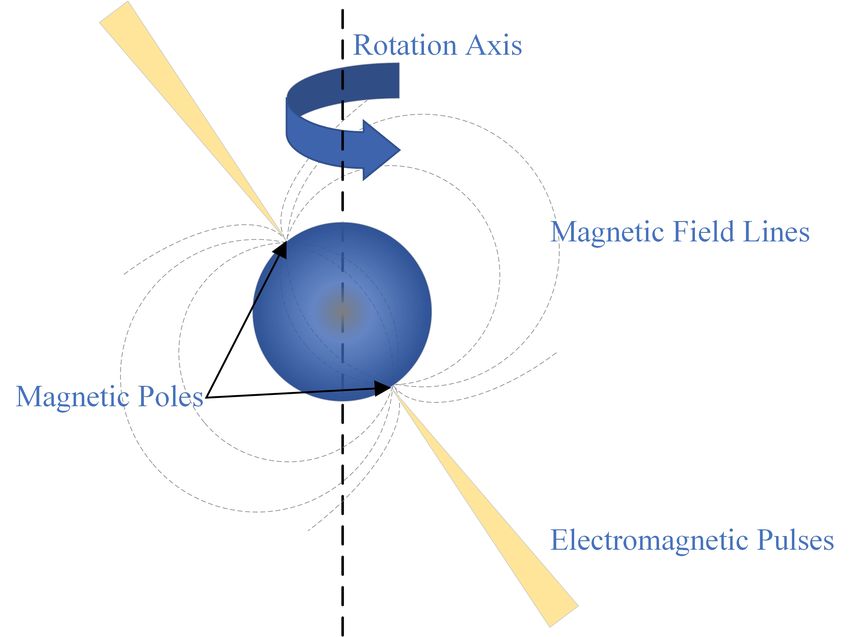
Entropy 2021, 23, 1181                                                                                          2 of 13

                         are the perfect choice for precise timing and autonomous interplanetary navigation [8–11].
                         The precise timing properties of pulsars can be used for unmanned out-terrestrial vehicles,
                         for instance, incorporating advanced robust control algorithms, such as those reported
                         in [12,13], with the pulsar TOA sequence as well as the pulsar positioning algorithm.
                         Nowadays, there are already over 2000 known pulsars that build a firm base for govern-
                         mental and civilian use, as well as space applications not only for the military but also for
                         astronomy exploration [14,15].
                               Among all types of pulsars, X-ray pulsars appear to be the most favorable ones as they
                         are detectable by small-size detectors [1,8,9,16–19]. However, the X-ray pulsar radiation,
                         namely the effective signals, would degenerate into photon sequences with very low
                         intensity when it arrives at the terrestrial detector after long-distance space travel. An
                         even more troublesome problem arises due to the complex, noisy photons, up to about
                         nine times that of the effective photons in quantity, including the diffuse X-ray background
                         and the cosmic X-ray background, which inherently contend with the originally observed
                         signal [11]. These facts imply the low signal-to-noise (SNR) ratio of the pulsar signal and,
                         hence, signify the necessity of pulsar denoising research, especially when the observation
                         time is short.
                               The pulsar denoising refers to filtering the pulsar profile, generally obtained via
                         epoch folding performed on photon sequences, that stores the time of arrivals (TOAs) of
                         photons [1,17,20]. The Fourier filtering in the frequency domain is the original attempt to
                         denoise pulsar profiles, which has already been proven invalid when the signal profile
                         comprises nonsinusoidal components or nongaussian noise [16,18,21]. The modified
                         kernel regression denoising method reported in [22] develops the second-order derivative
                         compensation and reveals that a clear positive relationship between the TOA accuracy and
                         the profile SNR does not exist. In [23], the wavelet analysis method using noise dispersion
                         to determine the threshold value is applied to denoise the pulsar profile via the wavelet
                         inverse transform. The denoising strategy based on biorthogonal lifting wavelet transforms
                         (WT) reported in [17] studied the statistical properties of the X-ray background noise. The
                         core idea of wavelet transform denoising is choosing an appropriate wavelet library and
                         decomposition level in terms of finding a suitable wavelet basis and threshold function [24].
                         In particular, the wavelet basis plays an essential role in denoising performance as it is
                         the base of wavelet denoising. However, at present, there is no universal wavelet basis
                         that accommodates different pulsar signals. It has also been shown in [21] that the wavelet
                         denoising methodology heavily relies on expertise and experience and is not compatible
                         with an average processor. New approaches to increase the SNR of X-ray pulsar signals
                         can be found in [25] with a machine learning method and in [26] with a recurrent neural
                         network method, respectively. These two kinds of denoising strategies actually require
                         high computational costs too.
                               Recently, empirical mode decomposition (EMD) has achieved great success in re-
                         moving both white and fractional Gaussian noise by reconstructing the signal with pre-
                         determined thresholding intrinsic mode functions (IMFs) [27]. Nevertheless, the traditional
                         EMD framework only allows for analyzing the single signal due to possible mixing phe-
                         nomena when analyzing multiple signals simultaneously. This problem can be overcome by
                         the multivariate strategy reported in [28], in which multiple pulsar signals are processed at
                         the time while the mode mixing is avoided. The ensemble empirical mode decomposition
                         (EEMD) synthesizes white Gaussian noise in the input signal for the later decomposition,
                         in which the average operation can also avoid the mode mixing problem that existed in the
                         output IMFs after EMD [29–31]. Given the limitation from the fixed threshold functions,
                         the adaptive threshold mechanism together with the EMD denoising method shown in [32]
                         remarkably increases the SNR of X-ray pulsar profiles. Via creating the Hausdorff measures
                         between the probability density functions of the input signal and the mode, the filtering
                         approach in [9] aliases and reconstructs the X-ray pulsar profiles to achieve the purpose of
                         denoising. Though the EMD framework allows for analyzing nonstationary and nonlinear
                         signals, it lacks a firm mathematical foundation and is sensitive to sampling noise, which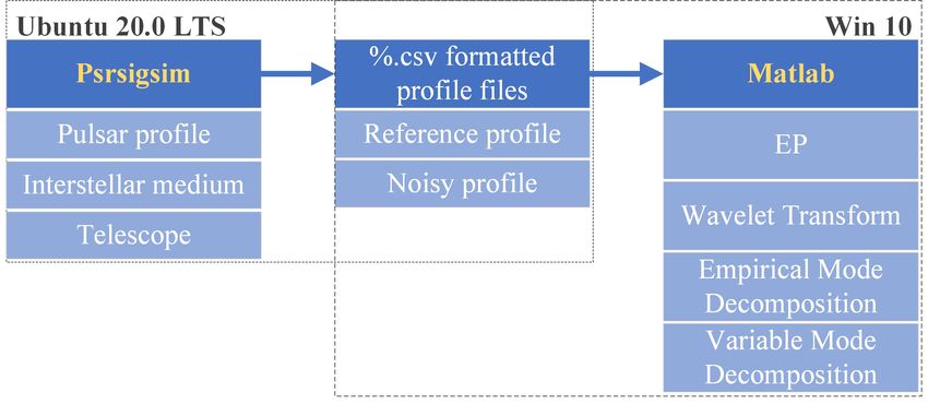
Entropy 2021, 23, 1181                                                                                            3 of 13

                         as a particular result, would lead to mode mixing when it is applied on pulsar denoising
                         processing. Additionally, one might find that eliminating the mode mixing problem would
                         build a firm base for performing autonomous mode decomposition and signal denoising,
                         which is essential for embedding advanced control algorithms, such as in [33], into the
                         pulsar-based spacecraft navigation system. Regarding the possible deficiencies of EMD on
                         pulsar signal denoising, Dragomiretskiy developed a novel signal decomposition technique
                         called variational mode decomposition (VMD) that nonrecursively decompose the signal
                         into several quasi-orthogonal IMFs [34]. The VMD has already been applied in many areas
                         such as seismic wave analysis [35], pipeline leakage detection [36] and vibration estimation
                         of rotor-stator machinery [37]. For VMD-based applications, it is important to determine an
                         accurate number of modes that have an essential effect on denoising performance [38]. The
                         detrended fluctuation analysis (DFA) appears to be a favorable choice for this issue as it is a
                         systematic scaling analysis approach to evaluate long-term dependency for nonstationary
                         signal series [35,36]. In our previous work [39], a brief VMD-based denoising algorithm
                         was developed for an X-ray pulsar profile after epoch folding without applying DFA to
                         determine the mode number. To the authors’ best knowledge, no literature reported had
                         shown a detailed discussion about applying the VMD framework on denoising X-ray
                         pulsar signals.
                              Motivated by the discussion above, this brief undertakes further endeavors on the
                         research of denoising designs of X-ray pulsar signals so as to increase the SNR of the
                         pulsar profiles and pave the way for potential applications. More precisely, a VMD-based
                         denoising strategy is developed. We first perform the epoch folding method on the faint
                         X-ray pulsar signals and obtain the noisy pulsar profile, followed by applying DFA to
                         obtain the number of IMFs, after which the reconstruction of the pulsar signals achieves
                         the denoising goal.
                              The contribution of this paper includes presenting the denoising algorithm for X-ray
                         pulsar signals based on the VMD method. Compared with those in [18,20,40], the prior
                         knowledge of pulsar profiles is unnecessary for the proposed VMD-based pulsar denoising
                         strategies. In comparison with wavelet analysis [17,23,24], the denoising algorithm in
                         this paper removes the reliance on choosing perfect basis and threshold functions. The
                         VMD-based design in this paper also allows for processing the original pulsar signals that
                         contain nonstationary background noise derived from many sources without leading to
                         mode mixing problems, like that of the EMD-based analysis in [9,28,32].
                              The rest of the paper is organized as follows. Section 2 introduces basic knowledge
                         of the VMD framework. Section 3 involves the VMD-based denoising design for the
                         contaminated faint X-ray pulsar signals. Section 4 presents the comparison experiments
                         with simulation and measured data. Section 5 concludes this work briefly.

                         2. Preliminaries
                         Variational Mode Decomposition
                               Variational Mode Decomposition (VMD) is a novel framework for signal processing
                         that outperforms the traditional decomposition approaches, allowing for a systematic
                         analysis of nonstationary and nonlinear signals [34]. It is built upon classical theories such
                         as the Wiener filter, Hilbert transformation, frequency mixing, and decomposition method.
                         Compared with the traditional empirical mode decomposition (EMD) technique, the VMD
                         theoretically eliminates the potential problem of mode mixing by decomposing the signal
                         into a sum of IMFs with the limited center frequency and bandwidth calculated analytically.
                         It is worth noting that the reconstruction of the VMD-based decomposed signals, namely
                         summing the obtained IMFs, would attenuate noise and increase SNR.
                               The VMD-based decomposition performed on the input signal f intends to achieve
                                                          (                                           )
                                                            K                                   2
                                                               ∂              1
                                                 min        ∑
                                               {hk },{ωk } k=1 ∂t
                                                                     δ(t) + j
                                                                              πt
                                                                                   ∗ hk (t) e − jωt
                                                                                                        ,            (1)
                                                                                                    2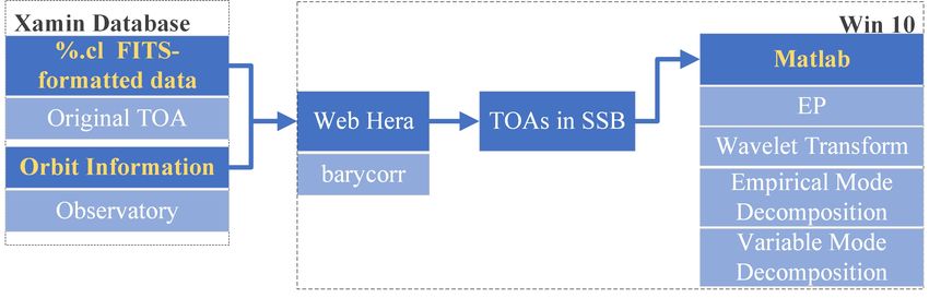
Entropy 2021, 23, 1181                                                                                                                          4 of 13

                                                                                             K
                         so that the f can be reconstructed by the sum ∑ hk = f , where {hk } and {ωk } denote the
                                                                                            k =1
                         sets of all modes and center frequencies, respectively; δ(t) stands for Dirac function and
                         notation ∗ denotes convolution. For definitions and discussions about the mode, refer
                         to [34,41]. For the sake of completeness and simplicity, the VMD algorithm renders the
                         constraint problem (1) into an unconstrained one via introducing a quadratic penalty term
                         α and Lagrangian multipliers λ(t), resulting in the following augmented Lagrangian.
                                                                          K                                                             2
                                                                                   ∂                            j
                                           L({hk }, {ωk }, λ) = α         ∑        ∂t
                                                                                             δ(t) +
                                                                                                               πt
                                                                                                                        ∗ hk (t) e− jωk t
                                                                      k =1                                                                  2

                                                                                        K                  2
                                                                 + f (t) −          ∑ hk (t)                                                       (2)
                                                                                    k =1                   2
                                                                     *                                               +
                                                                                                   K
                                                                 +        λ ( t ), f ( t ) −     ∑      hk (t) .
                                                                                                 k =1

                         It then converts the original minimization problem (1) into the saddle point problem of (2).
                         Iterative sub-optimizations in terms of the alternate direction multiplier method (ADMM)
                         can be used to obtain the saddle point of (2) and the optimal solution of (1). Let ωk and hi6=k
                         denote the most recently updated values, and the minimization problem for hnk +1 becomes
                                                                                                                                        2
                                                                 ∂                          j
                                            hnk +1   = arg min{α                    δ(t) +                          ∗ hk (t) e− jωk t
                                                         hk ∈ X  ∂t                        πt                                               2
                                                                                                       2                                           (3)
                                                                              λ(t)
                                                     + f ( t ) − ∑ hi ( t ) +                              }.
                                                                 t             2
                                                                                                       2

                             By applying the Parseval/Plancherel formula for Fourier transform together with
                         Hermitian properties under the L2 norm, we can find the optimal solution in the spectrum
                         domain as follows,
                                                                                   λ̂(ω )
                                                              fˆ(ω ) − ∑ ĥi (ω ) + 2
                                                                                            i6=k
                                                       ĥnk +1 (ω ) =                                                          .                   (4)
                                                                                   1 + 2α(ω − ωk )2
                         Implementing the same technical principles above, we obtain the center frequency in the
                         form of
                                                               R∞              2
                                                        n +1    0 ω ĥk ( ω ) dω
                                                      ωk = R                 2
                                                                                 .                            (5)
                                                                  ∞
                                                                 0 ĥk ( ω ) dω

                             The specific calculation steps of variational mode decomposition, intuitively including
                         denoising functionality, can be summarized as follows.
                         1.   Initialization: h1k , ω̂k1 , λ̂1 , n ← 0;
                         2.   n ← n + 1;
                         3.   Update ĥk and ωk via (4) and (5), respectively, where k = 1, 2, . . . , k, ∀ω ≥ 0;
                         4.   Use λ̂n+1 (ω ) = λ̂n (ω ) + τ [ fˆ(ω ) − ∑ ĥnk +1 (ω )] and update λ̂, ∀ω ≥ 0;
                                                                               k
                                                                                        2
                                                          K     ĥnk +1   − ĥnk
                                                                                        2
                         5.   Stop the iteration until ∑                                    < ε for a chosen criterion ε, otherwise return
                                                         k =1         ĥnk
                              to step 2.
                              Actually, one should calculate an appropriate number of mode K before applying
                         VMD to decompose the input signals. For this sake, the DFA approach is applicable
                         to determine K as it can characterize different components contained in the signal and
                         provides us with a threshold functionality for the calculation of K [21,35,36].
Entropy 2021, 23, 1181 5 of 13
Remark 1. Adopting the same simulation conditions as our previous work [42], we perform here a
comparison experiment of EMD and VMD on decomposing the analog signal defined by
cos(20πt), ∀t ∈ [0, 0.5],
cos(20πt) + cos(6πt) + cos(120πt),
f (t) = (6)
∀t ∈ (0.5, 0.8],
cos 20πt , ∀t ∈ 0.8, 1 .
( ) ( ]
The simulation results are drawn in Figure 2. As shown in Figure 2a, the EMD decomposes
f (t) into four intrinsic mode functions and residue, leading to background signals mixing with
frequencies 10 and 60 Hz. This mixing phenomenon distorts the intrinsic mode functions obtained
later, lowering the signal decomposition performance. Comparing the results in Figure 2b with that
in Figure 2a, the VMD features its superiority by accurately decomposing f (t) into three types of
signals with different time frames and frequencies.
2 2
0
0
-2
0 0.1 0.2 0.3 0.4 0.5 0.6 0.7 0.8 0.9 1
-2
1
0 0.1 0.2 0.3 0.4 0.5 0.6 0.7 0.8 0.9 1
0
1
-1
0 0.1 0.2 0.3 0.4 0.5 0.6 0.7 0.8 0.9 1
1 0
0
-1 -1
0 0.1 0.2 0.3 0.4 0.5 0.6 0.7 0.8 0.9 1 0 0.1 0.2 0.3 0.4 0.5 0.6 0.7 0.8 0.9 1
1
1
0
-1 0
0 0.1 0.2 0.3 0.4 0.5 0.6 0.7 0.8 0.9 1
0.2 -1
0.1 0 0.1 0.2 0.3 0.4 0.5 0.6 0.7 0.8 0.9 1
0
-0.1 1
0 0.1 0.2 0.3 0.4 0.5 0.6 0.7 0.8 0.9 1
0.5
0
-0.02 0
-0.04 -0.5
0 0.1 0.2 0.3 0.4 0.5 0.6 0.7 0.8 0.9 1 0 0.1 0.2 0.3 0.4 0.5 0.6 0.7 0.8 0.9 1
(a) EMD-based decomposition result for f (t). (b) VMD-based decomposition result for f (t).
Figure 2. Decomposing results of f (t) via EMD and VMD.
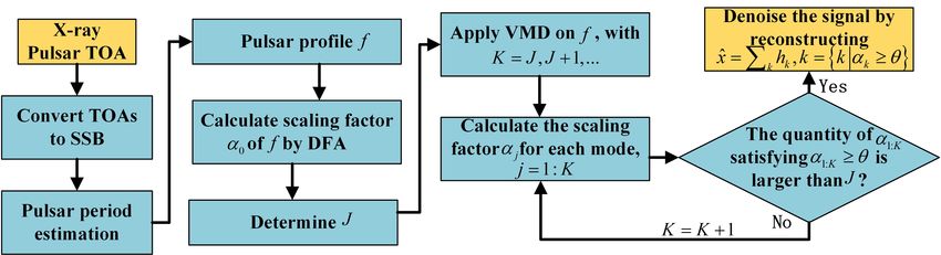
3. VMD-Based Denoising Design for X-ray Pulsar Signals
The X-ray pulsar signal observed by detectors contains the time of arrival and the
number of photons. It is contaminated by various types of electromagnetic noise. Denoising
X-ray pulsar signals appear essential for characterizing different pulsars and building a
base for accurate timing in space. In this section, we present a VMD-based denoising
method of X-ray pulsars step by step. First, we apply the epoch folding to obtain the noisy
pulsar profile. Second, we use the DFA approach to calculate the number of modes of the
pulsar profile. Third, we apply the VMD method to decompose and reconstruct the pulsar
profile, which achieves the purpose of denoising.
3.1. X-ray Pulsar Profile
Epoch folding is applied in this subsection to obtain the pulsar profile. Sort the TOAs
of photons into,
t00 ≤ t10 ≤ t20 ≤ . . . ≤ t0N −1 , (7)
where ti0 , i ∈ Z denotes the time of arrival of the i + 1-th photon. In (7), the symbol “≤”
suggests that numerous photons would run into the detector area simultaneously at a
certain observing window.Entropy 2021, 23, 1181 6 of 13
For eliminating the effects of earth-observatory motions and interstellar medium
during the pulsar signal transmitting path, we convert the TOAs of photons from observed
time tobs to the solar system barycenter (SSB) as follows,
tSSB = tobs + ∆E + ∆R + ∆S , (8)
where ∆E denotes Einstein delay, ∆R is the Roemer delay and ∆S represents the Shapiro
delay [43]. Many tools can be applied to finish the time conversion (8). For example, one
can synthesis tobs with the orbit parameters and evoke the barycorr function provided by
High Energy Astrophysics Science Archive Research Center (HEASARC) to complete the
time conversion automatically.
Denote the TOA sequences in SSB by
t 0 ≤ t 1 ≤ t 2 ≤ . . . ≤ t N −1 , (9)
Supposing that the pulsar period is T0 , the phase of (9) in the normalized time frame [0, 1)
with respect to the initial time instant can be calculated as
t i − t0
ϕi = mod 1. (10)
T0
Let us averagely scatter each period into m bins and compute the number of photons Ni in
each bin. Construct
m 2
( Ni − N̄ ) N
χ2 = ∑ , N̄ = . (11)
i =1
N̄ m
where N is the total number of photons, N̄ stands for the mean value of each bin. When
we only perform period estimation, the variable χ2 in (11) satisfies the χ2 -distribution with
m − 1 degrees of freedom. Different pulsar periods vary from phases and photon quantities
in each bin, which, as a result, shows that the obtained χ2 -distributions are different.
A period with errors would make the estimated phases inaccurate, simultaneously reducing
Ni , N̄ and χ2 . In contrast with that, an accurate estimated period suggests that the estimated
phases are reliable, and Ni and N̄ will differ a lot from each other, which increases χ2 .
Therefore, achieving the best estimation of period T relates to finding the maximum
of χ2 . Let
T = argT∈[Tmin ,Tmax ] max{Ø2 }. (12)
The estimated phase of the arrival time of every photon is assigned to a certain bin
according to the pulsar period, resulting in the estimated pulsar profile. The relationship
between the phase and the number of photons in each bin is drawn. For instance, the
horizontal axis of the pulsar profile is the phase with multiple bins, while the vertical
axis denotes the number of photons. Theoretically speaking, the longer the observing
time frame and the more the photon quantity, the more accurate the pulsar profile would
become [17,20].
3.2. Denoise of Pulse Profile Based on VMD
Without causing any confusion, let f , defined below, be the pulse profile,
f = x + d, (13)
where x is the original pulsar signal, and d denotes noise.
The number of modes K should be determined before performing VMD on f . The
K plays an essential role in VMD decomposition, or in the view of this brief, the wrong
choice of K would lower the denoising performance. For these considerations, we apply
the detrended fluctuation analysis (DFA) method to determine K. The DFA is a favorable
scaling tool generally utilized to analyze nonstationary signals, by which the scalingEntropy 2021, 23, 1181 7 of 13
exponent α depicts how tough the signal performs, and a large α means that the volatility
is small [21]. The K can then be calculated according to α.
Given any signal {u(i ), i = 1, 2, . . . , N }, let us apply DFA to calculate α by the steps
below.
1. Calculate the sum
k
y(k) = ∑ u(i) − kū, k = 1, 2, . . . , N, (14)
i =1
N
1
where ū = N ∑ u ( i ).
i =1
2. Divide the sequence y(k) into Nn = ( N/n) nonoverlap length-of-n pieces. As for
each local trend, one can apply l-order polynomial to fit yn (k). For example, let l = 2
and define
y n ( k ) = a n k 2 + bn k + c n , (15)
where an , bn and cn denote constants.
3. Define the root-mean-square (RMS) function by
v
N
u
u1
F (n) = t
N ∑ [y(k) − yn (k)]2 . (16)
k =1
4. Finally, calculate the scaling exponent α by the least square regression approach as
follows,
ln( F (n)) = α ln(n) + C. (17)
The relationship between K and α can be understood in the sense that the quantity of
all scaling exponents α1:K under the constraint α1:K ≥ θ equals J, where θ = αθ = 0.25
denotes the threshold and αθ = 0.5 for the white Gaussian noise. Without losing generality,
we suppose that the noise of the pulsar signal received by probes satisfies the Gaussian
distribution.
The variable J is determined by αθ via,
1,
α0 ≤ 0.8
2, 0.8Entropy 2021, 23, 1181 8 of 13
Figure 3. The denoising process of VMD on X-ray pulsar signals.
Remark 2. The VMD approach provides a general framework for signal processing. In addi-
tion to X-ray pulsar denoising designs, various VMD-based applications, such as seismic wave
analysis [35], pipeline leakage testing [36] and machinery vibration research [37], have achieved
significant attention.
4. Experimental Analysis
This section presents the experimental study focusing on validating the effectiveness
of the proposed X-ray pulsar denoising strategies. Both simulated and measured data of
the X-ray pulsar are considered. For performance evaluation purposes, various measures,
including the Signal to Noise Ratio (SNR), Root-Mean-Square Error (RMSE), and Pearson’s
correlation coefficient (PCC), are considered as follows.
M
2
∑ x (i )
v
u 1 M [x(i) − x̂(i)]2
u
SNR = 10 log i =1
, RMSE = t ∑ ,
M
2 M i=1 x(i)2
∑ [ x (i ) − x̂ (i )]
i =1
M M M
M ∑ x (i ) x̂ (i ) − ∑ x (i ) ∑ x̂ (i )
i =1 i =1 i =1
PCC = s s 2 ,
M
M 2 M
M
2 2
M ∑ x (i ) − ∑ x (i ) M ∑ x̂ (i ) − ∑ x̂ (i )
i =1 i =1 i =1 i =1
where x (i ) denotes the nominal signal, x̂ (i ) represents the estimated denoised signal,
and M stands for the signal length. A higher SNR value or a lower RMSE value leads
to better denoising performance. The PCC in the range [−1, 1] is generally utilized to
address the linear relativity of paired variables. The larger PCC would suggest better
denoising performance.
4.1. Experiments of Simulation Data
For pulsar simulation purposes, we applied the Psrsigsim pulsar signal simulator to
construct a virtual reference X-ray pulsar profile and associated noisy pulsar profile. The
Psrsigsim is a python toolbox developed for simulating pulsar signals based on the known
and open databases. Parameters including pulsar profile type, interstellar medium, and
telescope information should be set before propagating the virtual pulsar signals. In our
settings, we saved the pulsar profile data in the portable ‘%.csv’ form and processed the data
via Matlab. Figure 4 depicts the overall production of propagating data and processing.
Figure 4. Experiment flow chart of Psrsigsim-propagated pulsar data.Entropy 2021, 23, 1181 9 of 13
We adopted the default pulsar profile ‘J1713 + 07474’ provided by Psrsigsim as the ref-
erence profile, by which the noisy pulsar profile is constructed via the ‘pulsar.make_pulse’
function of the Psrsigsim class with a 2000-s observing time. As a result, two million pulsar
events in terms of phases were obtained and taken as noisy pulsar signals. The reference
pulsar profile is plotted in Figure 5a, while the noisy profiles in the first 1000 samples are
drawn in Figure 5b. The vertical coordinate unit is omitted for the convenient processing
of simulation data. Two hundred thousand noisy samples were adopted to perform filter-
ing techniques that include epoch folding (EP), wavelet transform (WT), empirical mode
decomposition (EMD), and variational mode decomposition (VMD). It is worth noting that
the pulsar profile data after EP builds the base for the latter three approaches, or say, the
latter three ones use the folding profile as the input source to perform filtering.
2
Reference Profile 8 Reference Profile
1.8
6 Noisy Profile
1.6
4
1.4 2
1.2 0
1 -2
0 0.1 0.2 0.3 0.4 0.5 0.6 0.7 0.8 0.9 1 0 0.1 0.2 0.3 0.4 0.5 0.6 0.7 0.8 0.9 1
Phase Phase
(a) Reference pulsar profile obtained from Psrsigsim. (b) Noisy pulsar profile for experimental use.
Figure 5. The reference and noisy pulsar profile of simulation data.
For EP filtering, we divided the adopted 200,000 noisy data into 1000 bins per the
whole period, following the routine of (7)–(11), and depicted the folding results in Figure 6a.
For WT filtering, the Matlab widenoise function was applied to denoise the pulsar profile
after EP, and we decomposed the profile signal into three layers, after which the coefficients
with high frequencies were eliminated manually. The reconstructed filtered profile after
WT is shown in Figure 6b. For EMD filtering, the Matlab emd function was directly applied
to process the EP-folded profile data sequence, and eight IMFs were obtained in which
the last seven ones were summed together to reconstruct the profile signal, as plotted in
Figure 6c. Finally, we implemented the proposed VMD-based denoising strategy to denoise
the EP-folded profile data and plotted the results in Figure 6d. For VMD decomposition,
we determined the mode number K = 3 via the DFA, as shown in (13)–(19), after which
the VMD function shown in [34] is evoked.
As shown in Figure 5b, the noisy pulsar profile lacks basic profile shape features,
which are important to characterize the pulsar property. Figure 6a–d demonstrates the
denoising performance of the EP, WT, EMD, and VMD, respectively. Compared with
the other three methods, it can be found that our VMD-based denoising strategy obtains
better denoising results, as the denoised profile features a more fluent shape and fewer
disturbances. For supporting this viewpoint, the SNRs, RMSEs, and PCCs of the original
noisy profile and the denoised profile samples are shown in Table 1.
Table 1. Denoising performance with simulation data.
Method ORI EP WT EMD VMD
SNR −0.1145 22.8210 25.9410 27.2745 29.8821
RMSE 1.0121 0.0727 0.0508 0.0435 0.0313
PCC 0.1554 0.8619 0.9251 0.9441 0.9668
In Table 1, the term ‘ORI’ refers to the original noisy profile samples. As can be seen, all
denoising methods chosen for comparison dramatically increase the SNR values compared
with the original profiles of negative SNR, which means that the pulsar signal intensity is
less than 1/10 of the noise. In particular, our VMD-based denoising strategy outperformsEntropy 2021, 23, 1181 10 of 13
the compared methods as it gained the highest SNR, smallest RMSE, and largest PCC
among the others.
2.5
2
Reference Profile Reference Profile
2 Profile after EP 1.8 Profile after WT
1.6
1.5
1.4
1 1.2
1
0.5
0 0.1 0.2 0.3 0.4 0.5 0.6 0.7 0.8 0.9 1 0 0.1 0.2 0.3 0.4 0.5 0.6 0.7 0.8 0.9 1
Phase Phase
(a) Pulsar profile after EP. (b) Pulsar profile after WT.
2 2
Reference Profile 1.8
Reference Profile
1.8
Profile after EMD Profile after VMD
1.6 1.6
1.4 1.4
1.2 1.2
1 1
0 0.1 0.2 0.3 0.4 0.5 0.6 0.7 0.8 0.9 1 0 0.1 0.2 0.3 0.4 0.5 0.6 0.7 0.8 0.9 1
Phase Phase
(c) Pulsar profile after EMD. (d) Pulsar profile after VMD.
Figure 6. Denoising results of simulation data via different methods.
4.2. Experiments of HEASARC-Archived Data
The real pulsar TOA data are implemented in this subsection to validate the pro-
posed pulsar denoising strategy. We chose the ni1011010301.cl file to perform denoising
experiments from the XAMIN database. The chosen ‘%.cl’ file includes the TOAs of Crab
Pulsar photons observed and archived by the NICER mission in standard FITS format.
The ni1011010301.cl file was created on 20 November 2017 after a 99-min continuous
observation of the Crab X-ray Pulsar and includes 1,680,000 observed photons.
Because the motions of earth and observatory, as well as the interstellar medium,
would distort the pulsar signals, we needed to convert the recorded TOAs to the solar
system barycenter (SSB). More precisely, the Web Hera, an online HEASARC HEAsoft
toolbox set, was applied to evoke the barycorr function that converts the TOA information
in ‘%.cl’ files into TOA in SSB, in which the associated orbit information should be set
simultaneously. Later on, we performed denoising analysis via EP, WT, EMD, and VMD,
respectively. The overall process is depicted in the Figure 7.
Figure 7. Experiment flow chart of HEASARC-archived pulsar data.
According to (12), we estimated the pulsar period by the Chi-square period estimation
method. The estimated pulsar period is 0.033742389697 s. As the SNR value becomes large
due to an increase in time frames used for folding, we view the pulse profile created by
all 1,680,000 observed data as the reference signal while viewing the pulse profile created
by the former 40,000 photons as a disturbance signal for experimental use. The reference
profile is then obtained by multiplying the nominal signal by the ratio of noisy photonEntropy 2021, 23, 1181 11 of 13
quantity and all photons, in which the phase part is divided into 100 bins. The reference
and noisy profiles are depicted in Figure 8a,b.
600 1000
Photon Numbers
Photon Numbers
Reference Profile Reference Profile
550 800
Noisy Profile
500 600
450 400
400 200
350 0
0 0.1 0.2 0.3 0.4 0.5 0.6 0.7 0.8 0.9 1 0 0.1 0.2 0.3 0.4 0.5 0.6 0.7 0.8 0.9 1
Phase Phase
(a) (b)
Figure 8. The reference and noisy pulsar profile archived pulsar data. (a) Reference pulsar profile
obtained via folding all photons; (b) Noisy pulsar profile.
The EP method was firstly used to obtain the X-ray pulsar profile, and the results
are shown in Figure 9a. Note that the obtained profile in Figure 9a includes 400 times
of folding because the total photon quantity in use is 40,000, and each period is divided
into 100 bins. For WT filtering, we followed the same routine as the previous subsection
and manually removed the high-frequency part, and the results are depicted in Figure 9b.
For EMD filtering, the EP-folded profile data were decomposed into six modes, and we
summed the later five ones to reconstruct the profile. The EMD-based denoising result is
shown in Figure 9c. For VMD filtering, we applied the method of (13)–(18) to calculate the
number of modes and obtain K = 3, based on which we performed VMD decomposition
and signal reconstruction. The VMD-based denoising results are shown in Figure 9d.
600 600
Photon Numbers
Photon Numbers
Reference Profile Reference Profile
Profile after EP Profile after WT
500 500
400 400
300 300
0 0.1 0.2 0.3 0.4 0.5 0.6 0.7 0.8 0.9 1 0 0.1 0.2 0.3 0.4 0.5 0.6 0.7 0.8 0.9 1
Phase Phase
(a) Pulsar profile after EP. (b) Pulsar profile after WT.
600 600
Photon Numbers
Photon Numbers
Reference Profile Reference Profile
550
Profile after EMD Profile after VMD
500
500
450
400
400
300 350
0 0.1 0.2 0.3 0.4 0.5 0.6 0.7 0.8 0.9 1 0 0.1 0.2 0.3 0.4 0.5 0.6 0.7 0.8 0.9 1
Phase Phase
(c) Pulsar profile after EMD. (d) Pulsar profile after VMD.
Figure 9. Denoising results of archived pulsar data via different methods.
It is observed from Figure 9a–d that the adopted approaches achieve denoising at
different levels. Figure 9c depicts the results after EP, in which obvious saw signals exist,
even though the pulse shape matches that of the reference. It is hard to distinguish the
best denoising algorithm among WT, EMD, and VMD from the plotted figures. We then
numerically summarized the SNRs, RMSEs, and PCCs of the denoised signals in the
following table for better comparisons.
The performance indexes in Table 2 indicate that all chosen experimental approaches
have realized denoising purposes, and the SNRs are obviously increased compared with
the original noisy signal. In particular, the proposed VMD-based denoising algorithm
outperforms the other three approaches when inputting virtual Psrsigsim-propagated
pulsar data. The obtained experimental results validate the effectiveness of the proposed
VMD-based X-ray pulsar denoising design.Entropy 2021, 23, 1181 12 of 13
Table 2. Denoising performance with measured data.
Method Ori EP WT EMD VMD
SNR 7.8000 25.9117 27.9890 29.1157 30.3373
RMSE 0.4132 0.0506 0.0391 0.0339 0.0270
PCC 0.0462 0.8748 0.9138 0.9277 0.9480
5. Conclusions
This paper has made further efforts on X-ray pulsar denoising techniques. The VMD
approach incorporated with EP and DFA is facilitated to derive a novel pulsar denoising
algorithm that features filtering capacity while eliminating the mode mixing problem after
EMD decomposition. Experimental results with both simulation and HEASARC-archived
pulsar data demonstrate that the proposed denoising algorithm outperforms the EP-, WT-
and EMD-based denoising approaches. In the future, the authors will apply the proposed
denoising algorithm on pulsar identification and pulsar-based navigation simulation of
orbital satellites.
Author Contributions: Conceptualization, Q.C. and Y.Z.; methodology, Q.C., Y.Z. and L.Y.; software,
Y.Z. and L.Y.; validation, Y.Z. and L.Y.; formal analysis, Q.C., Y.Z. and L.Y.; investigation, Q.C.,
Y.Z. and L.Y.; resources, Q.C., Y.Z. and L.Y.; data curation, Y.Z. and L.Y.; writing—original draft
preparation, L.Y.; writing—review and editing, L.Y.; visualization, L.Y.; supervision, L.Y.; project
administration, L.Y.; funding acquisition, Q.C. All authors have read and agreed to the published
version of the manuscript.
Funding: This work was supported by National Key R&D Program of China (No.2017YFB0503304).
Data Availability Statement: The HEASARC-archived %.cl file is available at https://heasarc.gsfc.
nasa.gov (accessed on 20 November 2017).
Conflicts of Interest: The authors declare no conflict of interest.
References
1. Xue, M.; Li, X.; Fu, L.; Liu, X.; Sun, H.; Shen, L. Denoising of X-ray pulsar observed profile in the undecimated wavelet domain.
Acta Astronaut. 2016, 118, 1–10. [CrossRef]
2. Buhler, R.; Blandford, R. The surprising crab pulsar and its nebula: A review. Rep. Prog. Phys. 2014, 77, 066901. [CrossRef]
3. DeLaney, T.; Weatherall, J. Model for deterministic chaos in pulsar radio signals and search for attractors in the Crab and Vela
pulsars. Astrophys. J. 1999, 519, 291. [CrossRef]
4. Hankins, T.; Kern, J.; Weatherall, J.; Elike, J. Nanosecond radio bursts from strong plasma turbulence in the Crab pulsar. Nature
2003, 422, 141–143. [CrossRef] [PubMed]
5. Schembri, F.; Sapuppo, F.; Bucolo, M. Experimental classification of nonlinear dynamics in microfluidic bubbles’ flow. Nonlinear
Dyn. 2012, 67, 2807–2819. [CrossRef]
6. Bucolo, M.; Grazia, F.D.; Sapuppo, F.; Virzi, M.C. A new approach for nonlinear time series characterization. In Proceedings of
the 2008 16th Mediterranean Conference on Control and Automation, Ajaccio, France, 25–27 June 2008.
7. Bonasera, A.; Bucolo, M.; Fortuna, L.; Frasca, M.; Rizzo, A. A new characterization of chaotic dynamics: The d∞ parameter.
Nonlinear Phenom. Complex Syst. 2003, 6, 779–786.
8. Shuai, P.; Chen, S.; Wu, Y.; Zhang, C.; Li, M. Navigation principles using X-ray pulsars. J. Astronaut. 2007, 28, 1538–1543.
9. Wang, L.; Zhang, S.; Lu, F. Pulsar signal denoising method based on empirical mode decomposition and independent component
analysis. In Proceedings of the 2018 Chinese Automation Congress (CAC), Xi’an, China, 30 November–2 December 2018;
pp. 3218–3221.
10. Buist, P.J.; Engelen, S.; Noroozi, A.; Sundaramoorthy, P.; Verhagen, S.; Verhoeven, C. Overview of pulsar navigation: Past, present
and future trends. Navigation 2011, 58, 153–164. [CrossRef]
11. Sun, J.; Xu, L.; Wang, T. New denoising method for pulsar signal. J. Xidian Univ. 2010.
12. Jia, Y. General solution to diagonal model matching control of multiple-output-delay systems and its applications in adaptive
scheme. Prog. Nat. Sci. 2009, 19, 79–90. [CrossRef]
13. Jia, Y. Robust control with decoupling performance for steering and traction of 4WS vehicles under velocity-varying motion.
IEEE Trans. Control. Syst. Technol. 2000, 8, 554–569.
14. Lan, S.; Xu, G.; Zhang, J. Interspacecraft ranging for formation flying based on correlation of pulsars. Syst. Eng. Electron. 2010, 3,
650–654.
15. Dahal, P. Review of pulsar timing array for gravitational wave research. J. Astrophys. Astron. 2020, 41, 8. [CrossRef]Entropy 2021, 23, 1181 13 of 13
16. Xie, Q.; Xu, L.; Zhang, H. X-ray pulsar signal detection using photon interarrival time. J. Syst. Eng. Electron. 2013, 24, 899–905.
[CrossRef]
17. Xue, M.; Li, X.; Liu, Y.; Fang, H.; Sun, H.; Shen, L. Denoising of X-ray pulsar observed profile using biorthogonal lifting wavelet
transform. J. Syst. Eng. Electron. 2016, 27, 514–523. [CrossRef]
18. Liang, H.; Zhan, Y. A fast detection algorithm for the X-ray pulsar signal. Math. Probl. Eng. 2017, 2017, 9607821. [CrossRef]
19. Mitchell, J.; Winternitz, L.; Hassouneh, M.; Price, S.; Semper, S.; Yu, W.; Ray, P.; Wolf, M.; Kerr, M.; Wood, K. Sextant X-ray pulsar
navigation demonstration: Initial on-orbit results. In Proceedings of the American Astronautical Society 41st Annual Guidance
and Control Conference, Breckenridge, CO, USA, 1–7 February 2018.
20. Su, Z.; Wang, Y.; Xu, L.-P.; Luo, N. A new pulsar integrated pulse profile recognition algorithm. J. Astronaut. 2010, 31, 1563–1568.
21. Li, F.; Zhang, B.; Verma, S.; Marfurt, K. Seismic signal denoising using thresholded variational mode decomposition. Explor.
Geophys. 2018, 49, 450–461. [CrossRef]
22. Song, J.; Qu, J.; Xu, G. Modified kernel regression method for the denoising of X-ray pulsar profiles. Adv. Space Res. 2018, 62,
683–691. [CrossRef]
23. Garvanov, I.; Iyinbor, R.; Garvanova, M.; Geshev, N. Denoising of pulsar signal using wavelet transform. In Proceedings of the
2019 16th Conference on Electrical Machines, Drives and Power Systems (ELMA), Varna, Bulgaria, 6–8 June 2019; pp. 1–4.
24. You, S.; Wang, H.; He, Y.; Xu, Q.; Feng, L. Frequency domain design method of wavelet basis based on pulsar signal. J. Navig.
2020, 73, 1223–1236. [CrossRef]
25. Singh, A.; Pathak, K. A machine learning-based approach towards the improvement of snr of pulsar signals. arXiv 2020,
arXiv:2011.14388.
26. Jiang, Y.; Jin, J.; Yu, Y.; Hu, S.; Wang, L.; Zhao, H. Denoising method of pulsar photon signal based on recurrent neural network.
In Proceedings of the 2019 IEEE International Conference on Unmanned Systems (ICUS), Beijing, China, 17–19 October 2019;
pp. 661–665.
27. Huang, N.; Shen, Z.; Long, S.R.; Wu, M.C.; Shih, H.; Zheng, Q.; Yen, N.; Tung, C.; Liu, H. The empirical mode decomposition and
the hilbert spectrum for nonlinear and non-stationary time series analysis. Proc. R. Soc. Lond. 1998, 454, 903–995. [CrossRef]
28. Jin, J.; Ma, X.; Li, X.; Shen, Y.; Huang, L.; He, L. Pulsar signal de-noising method based on multivariate empirical mode
decomposition. In Proceedings of the 2015 IEEE International Instrumentation and Measurement Technology Conference (I2MTC)
Proceedings, Pisa, Italy, 11–14 May 2015; pp. 46–51.
29. Caesarendra, W.; Kosasih, P.; Tieu, A.; Moodie, C.; Choi, B. Condition monitoring of naturally damaged slow speed slewing
bearing based on ensemble empirical mode decomposition. J. Mech. Sci. Technol. 2013, 27, 2253–2262. [CrossRef]
30. Wu, Z.; Huang, N. Ensemble empirical mode decomposition: A noise-assisted data analysis method. Adv. Adapt. Data Anal. 2009,
1, 1–41. [CrossRef]
31. Wang, L.; Shao, Y. Fault feature extraction of rotating machinery using a reweighted complete ensemble empirical mode
decomposition with adaptive noise and demodulation analysis. Mech. Syst. Signal Process. 2020, 138, 106545. [CrossRef]
32. Li, X.; Jin, J.; Wang, M.; Liu, Y.; Shen, Y. X-ray pulsar signal denoising based on emd with adaptive thresholding. In Proceedings
of the 2014 IEEE International Instrumentation and Measurement Technology Conference (I2MTC) Proceedings, Montevideo,
Uruguay, 12–15 May 2014; pp. 977–982.
33. Jia, Y. Alternative proofs for improved LMI representations for the analysis and the design of continuous-time systems with
polytopic type uncertainty: A predictive approach. IEEE Trans. Autom. Control 2003, 48, 1413–1416.
34. Dragomiretskiy, K.; Zosso, D. Variational mode decomposition. IEEE Trans. Signal Process. 2013, 62, 531–544. [CrossRef]
35. Liu, Y.; Yang, G.; Li, M.; Yin, H. Variational mode decomposition denoising combined the detrended fluctuation analysis. Signal
Process. 2016, 125, 349–364. [CrossRef]
36. Lu, J.; Yue, J.; Zhu, L.; Li, G. Variational mode decomposition denoising combined with improved bhattacharyya distance.
Measurement 2020, 151, 107283. [CrossRef]
37. Wang, Y.; Markert, R.; Xiang, J.; Zheng, W. Research on variational mode decomposition and its application in detecting
rub-impact fault of the rotor system. Mech. Syst. Signal Process. 2015, 60, 243–251. [CrossRef]
38. Lian, J.; Liu, Z.; Wang, H.; Dong, X. Adaptive variational mode decomposition method for signal processing based on mode
characteristic. Mech. Syst. Signal Process. 2018, 107, 53–77. [CrossRef]
39. Zhao, Y.; Jia, Y.; Chen, Q. Denoising of X-Ray Pulsar Signal Based on Variational Mode Decomposition. In Chinese Intelligent
Systems Conference; Springer: Singapore, 2020; pp. 419–427.
40. Garvanov, I.; Garvanova, M.; Kabakchiev, C. Pulsar signal detection and recognition. In Proceedings of the Eighth International
Conference on Telecommunications and Remote Sensing, Rhodes, Greece, 16–17 September 2019; pp. 30–34.
41. El, S.; Alexandre, R.; Boudraa, A. Analysis of intrinsic mode functions: A pde approach. IEEE Signal Process. Lett. 2009, 17,
398–401.
42. Zhao, Y. On the Denoising of X-ray Pulsar Signals. Bachelor’s Thesis, Beihang University, Beijing, China, 2020.
43. Shen, L. Research on the X-ray Pulsar Navigation. Bachelor’s Thesis, Xidian University, Xi’an, China, 2017.You can also read