The VISCACHA survey III. Star clusters counterpart of the Magellanic Bridge and Counter-Bridge in 8D - Star clusters counterpart of the ...
←
→
Page content transcription
If your browser does not render page correctly, please read the page content below
A&A 647, L9 (2021)
https://doi.org/10.1051/0004-6361/202040015                                                                           Astronomy
c ESO 2021                                                                                                             &
                                                                                                                      Astrophysics

                                                           LETTER TO THE EDITOR

                                                 The VISCACHA survey
III. Star clusters counterpart of the Magellanic Bridge and Counter-Bridge in 8D?
        B. Dias1 , M. S. Angelo2 , R. A. P. Oliveira3 , F. Maia4 , M. C. Parisi5,6 , B. De Bortoli7,8 , S. O. Souza3 ,
 O. J. Katime Santrich9 , L. P. Bassino7,8 , B. Barbuy3 , E. Bica10 , D. Geisler11,12,13 , L. Kerber9 , A. Pérez-Villegas3,14 ,
                           B. Quint15 , D. Sanmartim16 , J. F. C. Santos Jr.17 , and P. Westera18

        1
            Instituto de Alta Investigación, Sede Esmeralda, Universidad de Tarapacá, Av. Luis Emilio Recabarren 2477, Iquique, Chile
            e-mail: bdiasm@academicos.uta.cl
        2
            Centro Federal de Educação Tecnológica de Minas Gerais Av. Monsenhor Luiz de Gonzaga, 103, 37250-000 Nepomuceno, MG,
            Brazil
        3
            Universidade de São Paulo, IAG, Rua do Matão 1226, Cidade Universitária, São Paulo 05508-900, Brazil
        4
            Instituto de Física, Universidade Federal do Rio de Janeiro, 21941-972 Rio de Janeiro, RJ, Brazil
        5
            Observatorio Astronómico, Universidad Nacional de Córdoba, Laprida 854, X5000BGR Córdoba, Argentina
        6
            Instituto de Astronomía Teórica y Experimental (CONICET-UNC), Laprida 854, X5000BGR Córdoba, Argentina
        7
            Facultad de Ciencias Astronómicas y Geofísicas de la Universidad Nacional de La Plata, and Instituto de Astrofísica de La Plata
            (CCT La Plata – CONICET, UNLP), Paseo del Bosque s/n, B1900FWA La Plata, Argentina
        8
            Consejo Nacional de Investigaciones Científicas y Técnicas, Godoy Cruz 2290, C1425FQB Ciudad Autónoma de Buenos Aires,
            Argentina
        9
            Departamento de Ciências Exatas e Tecnológicas, UESC, Rodovia Jorge Amado km 16, 45662-900 Ilhéus, Brazil
       10
            Departamento de Astronomia, IF – UFRGS, Av. Bento Gonçalves 9500, 91501-970 Porto Alegre, Brazil
       11
            Departamento de Física y Astronomía, Universidad de La Serena, Avenida Juan Cisternas 1200, La Serena, Chile
       12
            Instituto de Investigación Multidisciplinario en Ciencia y Tecnología, Universidad de La Serena Benavente 980, La Serena, Chile
       13
            Departmento de Astronomía, Universidad de Concepción, Casilla 160-C, Concepción, Chile
       14
            Instituto de Astronomía, Universidad Nacional Autonóma de México, Apartado Postal 106, C.P. 22800 Ensenada, Baja California,
            Mexico
       15
            Gemini Observatory/NSF’s NOIRLab, Casilla 603, La Serena, Chile
       16
            Carnegie Observatories, Las Campanas Observatory, Casilla 601, La Serena, Chile
       17
            Departamento de Física, ICEx – UFMG, Av. Antônio Carlos 6627, Belo Horizonte 31270-901, Brazil
       18
            Universidade Federal do ABC, Centro de Ciências Naturais e Humanas, Avenida dos Estados, 5001, 09210-580 Santo André,
            Brazil

       Received 30 November 2020 / Accepted 26 February 2021

                                                                    ABSTRACT

       Context. The interactions between the Small and Large Magellanic Clouds (SMC and LMC) created the Magellanic Bridge; a stream
       of gas and stars pulled out of the SMC towards the LMC about 150 Myr ago. The tidal counterpart of this structure, which should
       include a trailing arm, has been predicted by models but no compelling observational evidence has confirmed the Counter-Bridge so
       far.
       Aims. The main goal of this work is to find the stellar counterpart of the Magellanic Bridge and Counter-Bridge. We use star clusters
       in the SMC outskirts as they provide a 6D phase-space vector, age, and metallicity which help characterise the outskirts of the SMC.
       Methods. Distances, ages, and photometric metallicities were derived from fitting isochrones to the colour-magnitude diagrams from
       the VISCACHA survey. Radial velocities and spectroscopic metallicities were derived from the spectroscopic follow-up using GMOS
       in the CaII triplet region.
       Results. Among the seven clusters analysed in this work, five belong to the Magellanic Bridge, one belongs to the Counter-Bridge,
       and the other belongs to the transition region.
       Conclusions. The existence of the tidal counterpart of the Magellanic Bridge is evidenced by star clusters. The stellar component of
       the Magellanic Bridge and Counter-Bridge are confirmed in the SMC outskirts. These results are an important constraint for models
       that seek to reconstruct the history of the orbit and interactions between the LMC and SMC as well as constrain their future interaction
       including with the Milky Way.
       Key words. Magellanic Clouds – galaxies: star clusters: general – galaxies: evolution

 ?
     Movie associated to Figs. 2, 3 and A.4 is available at https://www.aanda.org

                                                         Article published by EDP Sciences                                          L9, page 1 of 10
A&A 647, L9 (2021)

1. Introduction                                                        population detected by Harris (2007), who concluded that the
                                                                       Magellanic Bridge was formed only by gas, whereas stars were
The past interaction history between the Small and Large Mag-
                                                                       formed in situ. In this case, the compact spheroid should be a
ellanic Clouds (SMC, LMC) and of both galaxies with the Milky
Way has been a controversial topic of discussion in the last few       better choice, which poses a problem for the simulations. Nev-
                                                                       ertheless, Harris (2007) also found intermediate-age stars in the
decades. A canonical scenario describes the SMC and LMC as
                                                                       Bridge, but only in regions closer to the LMC and SMC, and
bound to the Milky Way for more than 5 Gyr, and it prescribes          they concluded that these stellar components are bound to their
that they only became a pair recently, meaning that the Magel-
                                                                       respective galaxies and not tidally stripped, because the old stars
lanic Stream and Leading Arm were formed from the interac-             are confined in the exponential surface density profile of the
tion among the three galaxies (e.g. Gardiner & Noguchi 1996;
Diaz & Bekki 2011, 2012). An alternative scenario describes the        LMC, before any break point. They did not analyse, in detail, the
                                                                       SMC Bridge population in the same way, presumably because of
Magellanic System as a bound SMC-LMC pair that is in its first
infall towards the Milky Way or at least in an elongated orbit         the complex geometry of the SMC. Nidever et al. (2011) applied
                                                                       a similar strategy and found a break point in the density profile
with a 6 Gyr period (e.g. Besla et al. 2007, 2010). In both cases,
simulations are able to roughly reproduce the large-scale gas          coincident with the same threshold of the ‘pure-bridge’ defined
                                                                       by Harris (2007) at about RA ∼ 2.5h . Therefore, the stellar coun-
structure of the Magellanic Stream and Leading Arm, traced by
HI gas (e.g. Putman et al. 1998; Nidever et al. 2008), the Mag-        terpart of the Magellanic Bridge (and Counter-Bridge, as a con-
                                                                       sequence) is indeed a tidally stripped population from the SMC
ellanic gaseous bridge (e.g. Hindman et al. 1963; Harris 2007),
and the old RR Lyrae bridge (e.g. Jacyszyn-Dobrzeniecka et al.         and may be of an old or intermediate age as proposed by the
                                                                       simulations of Diaz & Bekki (2012).
2017; Belokurov et al. 2017). However, the smaller structures               The old stellar tracers above are usually red clump stars
still need further simulations to fine-tune the most recent obser-
                                                                       which are useful for overall maps. A more comprehensive
vational constraints. This task is particularly challenging for
the complex structure of the SMC that is falling apart with a          picture can be obtained using star clusters as probes, repre-
                                                                       sented by a 6D phase-space vector, age, and metallicity, build-
large line-of-sight depth which is not trivial to characterise (e.g.
Bekki & Chiba 2009; Besla et al. 2007; Besla 2011; Dias et al.         ing up an 8D map of the SMC outskirts. Glatt et al. (2010)
                                                                       derived ages from the colour-magnitude diagrams (CMDs) of
2016; Niederhofer et al. 2018; Zivick et al. 2018; De Leo et al.
                                                                       324 SMC clusters, but using shallow photometry from the MCPS
2020). More multi-dimensional observational constraints are            survey (Zaritsky et al. 2002), covering only clusters younger
required to help trace the disruption scenario of the SMC.             than ∼1 Gyr, and assuming a fixed distance and metallicity.
     An important observed feature of the SMC structure that           Piatti et al. (2015) analysed 51 Bridge clusters from the VMC
has been detected by different surveys is the large line-of-           survey (Cioni et al. 2011) and found a predominant young pop-
sight depth of the stellar distribution in the north-eastern SMC,      ulation (∼20 Myr), which presumably formed in situ, and an
revealing a population at the mean distance of the SMC at
                                                                       older counterpart (∼1.3 Gyr), and they conclude that the Bridge
about 62 kpc (de Grijs & Bono 2015; Graczyk et al. 2020) and
a foreground population at about 50 kpc (e.g. Nidever et al.           could be older than previously thought. However, they also
2013; Mackey et al. 2018; Omkumar et al. 2021). The fore-              assumed a fixed distance for all clusters. It remains an open
ground component is interpreted as being the stellar counter-          question whether the old population actually corresponds to the
part of the Magellanic Bridge (a.k.a. Bridge), detected only           foreground tidal stellar counterpart of the Magellanic Bridge.
between 2.5◦ and 5–6◦ from the SMC towards the LMC. If this            Crowl et al. (2001) derived the 3D positions, ages, and metal-
is a tidal structure, it would be expected that distance correlates    licities of 12 SMC clusters and found that the eastern SMC side
with velocity, which is an indication of what was found by the         contains younger and more metal-rich clusters and has a larger
spectroscopic studies of Dobbie et al. (2014) and De Leo et al.        line-of-sigh depth than the western side, which is in agreement
(2020). In addition, Pieres et al. (2017) also found a stellar over-   with other works. They endorsed the use of populous star clus-
density towards the north of the SMC, which is also interpreted        ters as probes of the SMC structure.
as a tidally stripped structure.                                            In this paper we seek to confirm the tidal stripping nature of
     Various simulations are able to reproduce some of the             the SMC Bridge and Counter-Bridge using low-mass star clus-
observed features above, but not entirely; they also make pre-         ters. These clusters have been observed within the VIsible Soar
dictions that should be further checked with future observations.      photometry of star Clusters in tApii and Coxi HuguA (VIS-
For example, Diaz & Bekki (2012) performed N-body simula-              CACHA) survey1 (Maia et al. 2019, hereafter Paper I; Dias et al.
tions, modelling the SMC as a rotating disc (representing the          2020) that has been collecting deep and resolved photomet-
HI gas) and a non-rotating spheroid (representing the old stellar      ric data for star clusters in the outskirts of the Magellanic
component). They were able to reproduce the Magellanic Stream          Clouds, which are more susceptible to be tidally stripped (e.g.
and Leading Arm, which formed ∼2 Gyr ago; they also repro-             Mihos & Hernquist 1994).
duced the Magellanic Bridge (including the bifurcation) and they
predicted a tidal counterpart of the Bridge, called the Counter-
Bridge, both formed ∼150 Myr ago (also predicted by other sim-         2. Photometric and spectroscopic data
ulations such as those by Gardiner & Noguchi 1996 and Besla            The VISCACHA photometric data used here were observed
2011, although with a different orientation, shape, extension, and     in 2016, 2017, and 2019 under programmes SO2016B-018,
density). Diaz & Bekki (2012) tested three truncation radii to         SO2017B-014, and SO2019B-019, using the ground-based
model the spheroid component, the extended model being pre-            4m telescope SOAR and its adaptive optics module SAM
ferred as it reproduces the morphology and velocity pattern of         (Tokovinin et al. 2016). Data reduction, PSF photometry, and
the Magellanic Bridge better as well as a density break point          CMD decontamination based on membership probability were
detected by Nidever et al. (2011) at about 7◦ from the SMC cen-        performed following the methodology presented in Paper I.
tre. This is a remnant of a merger event, although with a simu-            The spectroscopic data were observed in 2018 with GMOS,
lated position at ∼4◦ . On the other hand, this would imply that       Gemini-S, under the Chile-Brazil-Argentina joint programmes
the stellar counterpart of the Magellanic Bridge is old, which
                                                                       1
does not seem to be the case of the exclusively young stellar              http://www.astro.iag.usp.br/~viscacha/

L9, page 2 of 10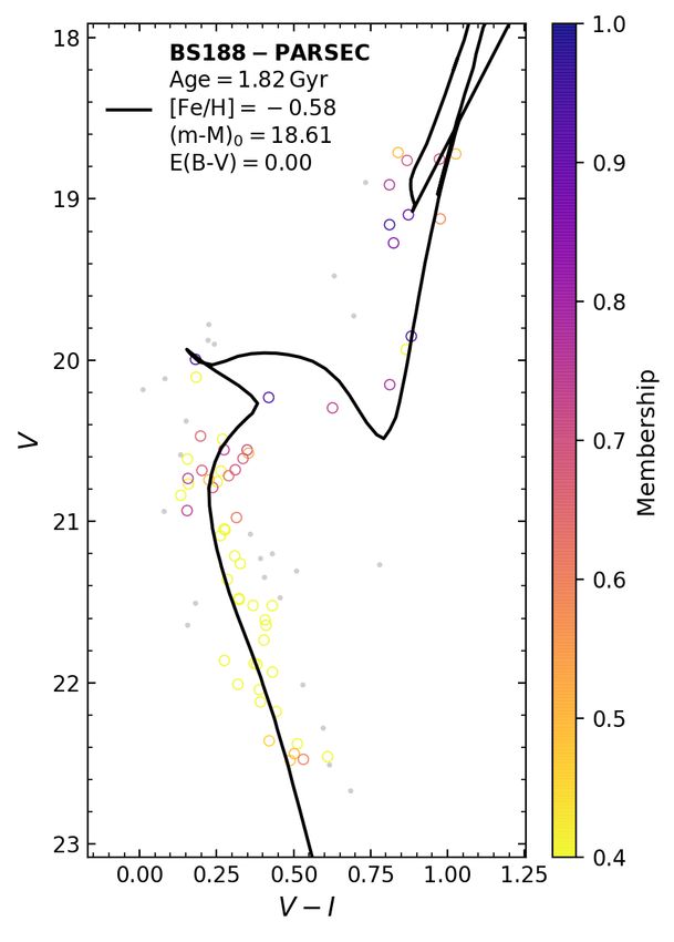
B. Dias et al.: The VISCACHA survey. III.

GS-2018B-Q-208 and GS-2018B-Q-302 to provide radial veloc-                                                              103
ities (RVs), a crucial parameter to characterise tidal tails. The                                                                                 ●   [2D,D14] Main body
                                                                                                                                                      [2D,D14] West Halo
data reduction was done using default tasks of the Gemini data                                                                ●
                                                                                                                                                      [2D,D14] Wing/Bridge

                                                                                                            (# deg−2)
reduction software, automated by a script developed and fine-                                                           102       ●                   [2D,D14] Counter−Bridge

tuned by M. S. Angelo2 . The 1D spectra were extracted, with                                                                          ●
                                                                                                                                          ●       inner region:

special attention to the wavelength calibration, that is to say                                                                                   log(dens) = 2.60(0.20) − 0.84(0.12) a

                                                                                       star cluster density
                                                                                                                        101                       outer region:
skylines were used as references along with the arc-lamps to

                                                                                                     NA
                                                                                                                                                  log(dens) = −0.05(0.47) − 0.06(0.05) a

enable absolute RV analysis. Proper motions were taken from
Gaia Early Data Release 3 (EDR3, Gaia Collaboration 2021a,                                                              100
see Appendix A.2).
                                                                                                              10−1
2.1. Statistical isochrone fitting
The CMD morphology of a star cluster depends on the age,                                                                      0           2   4       6          8          10             12
                                                                                                                                                  a Index
                                                                                                                                                    (deg)
metallicity, distance, and reddening. Therefore, it is mandatory
to fit all four parameters together to carry out a self-consistent       Fig. 1. SMC star cluster radial density profile (catalogued by Bica et al.
analysis. We used the SIRIUS code (Souza et al. 2020) that per-          2020), using the semi-major axis a of ellipses drawn around the SMC
forms a statistical isochrone fitting, with a Bayesian approach          centre as defined by D14 (see also Fig. 2), with 0.5◦ bins. Solid lines are
based on the Markov chain Monte Carlo sampling method. We                the fits to each region, whereas the dotted lines are extrapolation to find
adopted the geometrical likelihood function and the member-              the intersection at a = 3.4+1.0
                                                                                                    −0.6 , represented by the shaded grey 1σ area.
ship probability of stars as a uniform prior. The fits are blind         The arrows indicate the position of the seven clusters.
to spectroscopic metallicities, which were used to compare with
the photometric metallicities as a quality check of both indepen-
dent analyses.                                                           Massana et al. (2020), (ii) the break point by the simulations of
                                                                         Diaz & Bekki (2012), and (iii) with the vertex of the V inversion
                                                                         in the metallicity gradient (Parisi et al. 2015; Bica et al. 2020).
2.2. CaT analysis
                                                                         All seven clusters analysed in this paper are located around the
Radial velocities were derived by cross-correlation of the               break point or beyond it (see Table 1).
observed spectra of individual stars in the clusters against a tem-           The SMC boundary along the line-of-sight defined by the
plate synthetic spectrum from the library of Coelho (2014) with          simulation results of Diaz & Bekki (2012) is between ∼59 kpc
typical atmospheric parameters for red giant branch (RGB) stars,         and ∼65 kpc, which we adopted here as a first approximation to
that is (T eff , log(g), [Fe/H], [α/Fe]) = (5000 K, 1.0 dex, −1.0 dex,   identify five Bridge clusters and one (IC 1708) Counter-Bridge
0.4 dex). RVs and uncertainties were derived using fxcor at              cluster (see Table 1 and Fig. 2). The seventh cluster (Bruck 168)
IRAF, and the conversion from the observed velocities to RVhel           has a line-of-sight distance consistent with being bound to the
was calculated using rvcorrect at IRAF (Table 1). Spectroscopic          SMC; therefore, we placed this cluster in a transition region.
metallicities were derived following the recipes of Dias & Parisi        It is worth noting that the spheroid component of the Counter-
(2020), using a calibration of the reduced equivalent width of           Bridge (a.k.a. stars) is much less pronounced and less dense than
CaII triplet lines (CaT) with metallicity.                               the respective disc component (a.k.a. gas, see Omkumar et al.
    The membership selection follows the methodology by                  2021); as a result, it is not a surprise to find only a single repre-
Parisi et al. (2009). Briefly, stars within the cluster radius with      sentation of the Counter-Bridge in our cluster sample. Moreover,
an RV and [Fe/H] within windows of 10 km s−1 and 0.2 dex                 there seems to be a trend in the sense that north-eastern Bridge
around the group of innermost stars with a common RV and                 clusters are also closer to us (see Fig. 2), which supports the sce-
[Fe/H] are considered as members. The cluster radii were taken           nario that the foreground stellar population shapes the start of
from Santos et al. (2020), whenever available, or from Bica et al.       the Magellanic Bridge towards the LMC.
(2020) otherwise.                                                             Another crucial perspective is to analyse how these star clus-
                                                                         ters move with respect to the distance from the SMC in 3D space.
                                                                         Figure 3 shows how the RVs from the GMOS spectra and Gaia
3. Discussion                                                            EDR3 proper motions vary with the line-of-sight distance and
                                                                         projected distance on sky a. Tidally stripped structures show a
The starting point to discuss the SMC tidal tails is to argue            distance-velocity correlation, which characterises the Bridge and
whether a particular group of star clusters is bound or unbound          Counter-Bridge gas and stars very clearly (Gardiner & Noguchi
to the SMC. This is not trivial; however, Nidever et al. (2011)          1996, Fig. 11; Diaz & Bekki 2012, Figs. 9 and 15). In Fig. 3,
and Diaz & Bekki (2012) have argued that a sharp break in                we find a slope between RVhel and the line-of-sight distance of
the radial SMC stellar density distribution indicates tidal distor-      3.7±1.8 km s−1 kpc−1 , which is in good agreement with the slope
tions. Dias et al. (2014; 2016, hereafter D14,D16) divided the           of 3.4 km s−1 kpc−1 found by Gardiner & Noguchi (1996) in their
projected distribution of the SMC star cluster population that is        simulations and 4.0 km s−1 kpc−1 found by Mathewson et al.
outside the SMC main body (a > 2◦ ) into three regions (split            (1988) based on Cepheids. This agreement is interesting because
by voids in the azimuth direction) possibly related to differ-           Cepheids trace the younger stellar populations, which would
ent disrupting episodes: Wing and Bridge, Counter-Bridge, and            support a scenario where Bridge stars were formed in situ.
West Halo. We show in Fig. 1 that all regions share a similar            However, our Bridge and Counter-Bridge sample is composed
radial density profile, with a clear break point at a = 3.4◦+1.0
                                                              −0.6 ,
                                                                         of clusters with ages ranging from ∼1−4 Gyr, meaning that
which is consistent with (i) the SMC tidal radius rtSMC ∼ 4.5◦           these clusters were formed before the LMC-SMC encounter
and the break point for young and old populations found by               ∼150 Myr ago, which moved them from their original SMC
                                                                         orbits. Furthermore, Hatzidimitriou et al. (1993) found a slope
2
  http://drforum.gemini.edu/topic/                                       of 8 km s−1 kpc−1 based on red clump stars closer than 60 kpc,
gmos-mos-guidelines-part-1/                                              which would trace intermediate-age and older populations.
                                                                                                                                                                                           L9, page 3 of 10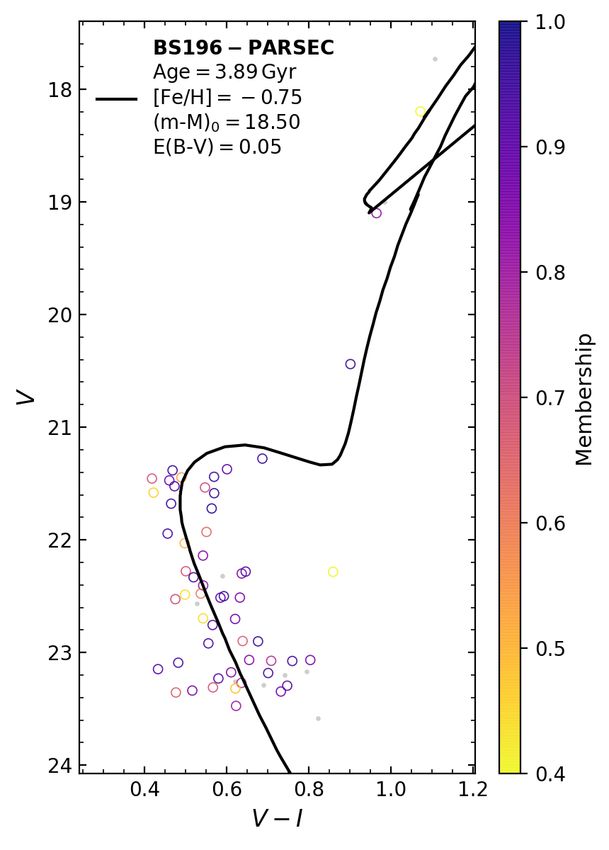
A&A 647, L9 (2021)
Table 1. Derived parameters for the star clusters.
Cluster Age [Fe/H]CMD [Fe/H]CaT E(B − V) Dist. a α J2000 δ J2000 RVhel µα · cos(δ) µδ
±unc.(std.dev.) ±unc.(std.dev.) ±unc.(std.dev.) ±unc.(std.dev.)
name (Gyr) (dex) (dex) (mag) (kpc) (deg) hh:mm:ss dd:mm:ss (km s−1 ) (mas yr−1 ) (mas yr−1 )
Magellanic Bridge
BS 196 3.89+0.68
−0.50
−0.75+0.22
−0.19 −0.89 ± 0.04(0.08) 0.05+0.04
−0.04 50.1+1.6
−2.2 5.978 01:48:01.8 −70:00:13 135.5 ± 1.4(2.7) 1.12 ± 0.07(0.18) −1.14 ± 0.06(0.05)
BS 188 (∗) 1.82+0.22
−0.20 −0.58+0.13
−0.13 −0.94 ± 0.06(0.13) 0.00+0.03
−0.00 52.7+3.0
−3.1 4.441 01:35:10.9 −71:44:11 120.3 ± 3.5(7.9) 1.25 ± 0.08(0.23) −1.35 ± 0.07(0.04)
HW 56 (∗∗) 3.09+0.22
−0.14 −0.54+0.07
−0.12 −0.97 ± 0.12(0.20) 0.03+0.02
−0.02 53.5+1.2
−1.2 2.397 01:07:41.1 −70:56:06 157.7 ± 5.4(9.3) 0.99 ± 0.11(0.04) −1.27 ± 0.10(0.29)
HW 85 1.74+0.08
−0.12 −0.83+0.07
−0.05
−0.82 ± 0.06(0.14) 0.04+0.02
−0.02 54.0+1.2
−2.0 5.219 01:42:28.0 −71:16:44 143.2 ± 3.0(6.8) 1.26 ± 0.09(0.47) −1.41 ± 0.09(0.26)
Lindsay 100 3.16+0.15
−0.14 −0.73+0.03
−0.03 −0.89 ± 0.06(0.14) 0.01+0.01
−0.01 58.6+0.8
−0.5
2.556 01:18:16.9 −72:00:06 145.8 ± 1.4(3.3) 0.98 ± 0.05(0.15) −1.10 ± 0.05(0.11)
Transition
+0.8
Bruck 168 6.6−0.9 −1.22+0.20
−0.15
−1.08 ± 0.06(0.09) 0.00+0.02
−0.01 61.9+2.3
−2.0 3.584 01:26:42.7 −70:47:01 141.7 ± 4.6(7.9) 0.94 ± 0.09(0.08) −1.15 ± 0.09(0.04)
Counter-Bridge
IC 1708 0.93+0.16
−0.04 −1.02+0.05
−0.10 −1.11 ± 0.06(0.17) 0.06+0.02
−0.02 65.2+1.2
−1.8 3.286 01:24:55.9 −71:11:04 214.9 ± 2.7(6.6) 0.39 ± 0.10(0.35) −1.26 ± 0.07(0.20)
Notes. Age, [Fe/H]CMD , E(B − V), distance from VISCACHA CMD isochrone fitting, [Fe/H]CaT , RVhel from GMOS spectra, µα , and µδ from Gaia
EDR3. Distance a follows the definition by Dias et al. (2014), and (α, δ) coordinates are from Bica et al. (2020). (∗) BS 188 was observed under sub-
optimal weather conditions, and the resulting isochrone fitting is very sensitive to a handful of stars from the shallow CMD, which could explain
the metallicity difference between photometric and spectroscopic [Fe/H] (see Appendix A.1). (∗∗) HW 56 is immersed in a dense field (a = 2.397◦ ,
the smallest in our sample) that has a very similar CMD as the cluster region; therefore, the statistical decontamination left low-probable member
stars on the fainter main sequence region, which may bias the photometric metallicities (see Appendix A.1). These uncertainties do not change the
conclusions of this work.
d=59.9(3.5)-1.51(1.40)
70 r2 = 0.07 -0.5
Bridge
Counter-Bridge
Transition
(mas yr 1)
-1.0
dist. (kpc)
[2D,D14] Main body
60 [2D,D14] West halo
[2D,D14] Wing/bridge -1.5
[2D,D14] Counter-bridge
[DB12] SMC bound
50
-2.0
6.0 2.0
4.0 Bridge
1.5
cos( ) (mas yr 1)
2.0
()
0.0
1.0
-2.0 2
=12.6(2.1)-0.20(0.04) d =1.8(0.5)-0.015(0.009) d
-4.0 4 r2 = 0.61 0.5 r2 = 0.37
10 8 6 Counter
-6.0 6.0 4.0 2.0 0.0 -2.0 -4.0 Bridge
50 60 70 300.0
0.0
cos ( ) dist. (kpc)
RVhel=-64(107)+3.7(1.8) d RVhel=170(25)-5.7(5.5) a
250.0 r2 = 0.50 r2 = 0.13
Fig. 2. Position of the seven star clusters in relative equatorial coor-
dinates as defined by D14, as seen in the planes (∆α,∆δ), (∆α,dist), 200.0
RVhel(km s 1)
and (∆δ,dist). Background points are all star clusters from Bica et al.
(2020). The seven clusters are located in the proposed ‘Counter-Bridge’ 150.0
2D projected region by D14, but we now show that this region actually 100.0
contains Bridge and Counter-Bridge clusters in 6D phase-space. The Counter
turquoise shaded area is a first approximation for the region bound to 50.0 Bridge Bridge
the SMC. Linear fits were performed for Bridge clusters only, consid- 0.0
ering the uncertainties. See Appendix A.3 for a 3D view of the clusters 50.0 60.0 70.0 0.0 1.0 2.0 3.0 4.0 5.0 6.0
dist. (kpc) a(deg)
and a movie is also provided online.
Fig. 3. 3D motion of the seven star clusters. Point colours and shaded
areas are the same as in Fig. 2. The black square marks the SMC sys-
A larger sample of clusters is required to compare the correla- temic motion and position (see Table A.1). Linear fits were performed
tion with this study. The correlation of RVhel with the projected considering the uncertainties and using all clusters to allow direct com-
distance a also reveals a trend in the sense that the Bridge clus- parison with other studies (see text). See Appendix A.3 for a 3D view
ters that are farther away from the SMC projected centre are of the clusters and a movie is also provided online.
also closer to us and dragging behind towards the LMC. These
results are consistent again with one branch of the Magellanic
Bridge starting in the north-eastern SMC. The Counter-Bridge constant. This is consistent with the scrutiny of Omkumar et al.
also starts in the same region, but so far we only have one point, (2021) on the simulations by Diaz & Bekki (2012) and also con-
and a larger sample would help constrain this tidal tail. Gaia sistent with the Gaia EDR3 proper motion distribution of the
EDR3 proper motions show relatively large error bars (Fig. 3); Magellanic System (see Appendix A.2).
nevertheless, the bulk of Bridge clusters are indeed separated Last but not least, concerning the eighth dimension anal-
from the Counter-Bridge cluster in µα , whereas µδ is roughly ysed here, we report that the metallicity of the five Bridge
L9, page 4 of 10B. Dias et al.: The VISCACHA survey. III.
Bridge Bridge
clusters (h[Fe/H]CMD i = −0.69 ± 0.12 dex; h[Fe/H]CaT i = study was financed in part by the Coordenação de Aperfeiçoamento de Pessoal
−0.90 ± 0.06 dex) is ∼0.2−0.3 dex, that is, ∼2σ higher than de Nível Superior – Brasil (CAPES) – Finance Code 001. A.P.V. and S.O.S.
acknowledge the DGAPA-PAPIIT grant IG100319. D.G. gratefully acknowl-
= −1.02+0.05
C.−Bridge
the Counter-Bridge cluster ([Fe/H]CMD −0.10 dex, edges support from the Chilean Centro de Excelencia en Astrofísica y Tec-
C.−Bridge
[Fe/H]CaT = −1.11 ± 0.06 ± 0.17 dex). Moreover, the Bridge nologías Afines (CATA) BASAL grant AFB-170002. D.G. also acknowledges
financial support from the Dirección de Investigación y Desarrollo de la Uni-
clusters are all older than the Counter-Bridge cluster. This sug- versidad de La Serena through the Programa de Incentivo a la Investigación
gests differences in metallicities per SMC region as indicated de Académicos (PIA-DIDULS). R.A.P.O. and S.O.S. acknowledge the FAPESP
by Crowl et al. (2001) and endorses further investigation. A pos- PhD fellowships nos. 2018/22181-0 and 2018/22044-3. The authors thank the
sible metallicity gradient would not eliminate this difference referee for the comments that improved this Letter.
because more distant Counter-Bridge clusters would have sim-
ilar metallicities (Parisi et al. 2015) or be even more metal-poor
(D14). References
Bekki, K., & Chiba, M. 2009, PASA, 26, 48
Belokurov, V., Erkal, D., Deason, A. J., et al. 2017, MNRAS, 466, 4711
4. Conclusions Besla, G. 2011, Ph.D. Thesis, Harvard University, USA
The gaseous complex structure of the Magellanic System and Besla, G., Kallivayalil, N., Hernquist, L., et al. 2007, ApJ, 668, 949
Besla, G., Kallivayalil, N., Hernquist, L., et al. 2010, ApJ, 721, L97
its stellar counterpart, in particular around the SMC, has been Bica, E., Santiago, B., Bonatto, C., et al. 2015, MNRAS, 453, 3190
observed and simulated by many previous works. We present Bica, E., Westera, P., Kerber, L. D. O., et al. 2020, AJ, 159, 82
an analysis of this question using star clusters observed within Cioni, M. R. L., Clementini, G., Girardi, L., et al. 2011, A&A, 527, A116
the VISCACHA survey. The advantage of this approach is that Coelho, P. R. T. 2014, MNRAS, 440, 1027
we are able to describe the Magellanic Bridge and Counter- Crowl, H. H., Sarajedini, A., Piatti, A. E., et al. 2001, AJ, 122, 220
Bridge in the 6D phase-space plus age and metallicity. We have de Grijs, R., & Bono, G. 2015, AJ, 149, 179
de Grijs, R., Wicker, J. E., & Bono, G. 2014, AJ, 147, 122
reached ∼1−6% precision in distance, ∼0.5−8% precision in De Leo, M., Carrera, R., Noël, N. E. D., et al. 2020, MNRAS, 495, 98
the mean RV, not to mention ∼4−20% precision in age, and Dias, B., & Parisi, M. C. 2020, A&A, 642, A197
∼0.03−0.22 dex and ∼0.04−0.12 dex precision in the mean pho- Dias, B., Kerber, L. O., Barbuy, B., et al. 2014, A&A, 561, A106
tometric and spectroscopic metallicities. Dias, B., Kerber, L., Barbuy, B., Bica, E., & Ortolani, S. 2016, A&A, 591, A11
From the seven clusters analysed here, we found that five Dias, B., Maia, F., Kerber, L., et al. 2020, IAU Symp., 351, 89
Diaz, J., & Bekki, K. 2011, MNRAS, 413, 2015
belong to the Magellanic Bridge, while one belongs to the Diaz, J. D., & Bekki, K. 2012, ApJ, 750, 36
Counter-Bridge and another is located at an intermediate region Dobbie, P. D., Cole, A. A., Subramaniam, A., & Keller, S. 2014, MNRAS, 442,
between the two tidal tails. Six-dimensional phase-space vectors 1663
of these clusters are consistent with the predictions from the sim- Gaia Collaboration (Brown, A. G. A., et al.) 2021a, A&A, in press, https:
ulations by Diaz & Bekki (2012), which confirms their unbound //doi.org/10.1051/0004-6361/202039657
current situation. These clusters are 1–4 Gyr old, therefore, they Gaia Collaboration (Luri, X., et al.) 2021b, A&A, in press, https://doi.org/
10.1051/0004-6361/202039588
were formed before the SMC-LMC close encounter that gener- Gardiner, L. T., & Noguchi, M. 1996, MNRAS, 278, 191
ated the SMC tidal tails and moved these clusters away from the Glatt, K., Grebel, E. K., & Koch, A. 2010, A&A, 517, A50
SMC main body. Graczyk, D., Pietrzynski, G., Thompson, I. B., et al. 2020, ApJ, 904, 13
The 2D projected SMC Counter-Bridge region as defined by Harris, J. 2007, ApJ, 658, 345
D14,D16 contains a mix of Bridge and Counter-Bridge clusters Hatzidimitriou, D., Cannon, R. D., & Hawkins, M. R. S. 1993, MNRAS, 261,
873
in a five-to-one ratio. Consequently, the Magellanic Bridge also Hindman, J. V., Kerr, F. J., & McGee, R. X. 1963, Aust. J. Phys., 16, 570
has a branch starting from the north-eastern SMC, in addition to Jacyszyn-Dobrzeniecka, A. M., Skowron, D. M., Mróz, P., et al. 2017, Acta
the eastern SMC wing and south-eastern RR Lyrae bridge. Astron., 67, 1
The present sample gives important hints on a likely scenario Kallivayalil, N., van der Marel, R. P., Besla, G., Anderson, J., & Alcock, C. 2013,
for the formation of a structure in the clouds, in particular the ApJ, 764, 161
Bridge and the Counter-Bridge. A larger sample is expected to Mackey, D., Koposov, S., Da Costa, G., et al. 2018, ApJ, 858, L21
Maia, F. F. S., Dias, B., Santos, J. F. C., et al. 2019, MNRAS, 484, 5702
further constrain the perturbed outskirts of the SMC. Massana, P., Noël, N. E. D., Nidever, D. L., et al. 2020, MNRAS, 498, 1034
Mathewson, D. S., Ford, V. L., & Visvanathan, N. 1988, ApJ, 333, 617
Acknowledgements. B.D. and M.C. Parisi acknowledge S. Vasquez for pro- Mihos, J. C., & Hernquist, L. 1994, ApJ, 425, L13
viding his code to measure CaT equivalent widths. Based on observations Nidever, D. L., Majewski, S. R., & Butler Burton, W. 2008, ApJ, 679, 432
obtained at the Southern Astrophysical Research (SOAR) telescope, which is Nidever, D. L., Majewski, S. R., Muñoz, R. R., et al. 2011, ApJ, 733, L10
a joint project of the Ministério da Ciência, Tecnologia, e Inovação (MCTI) da Nidever, D. L., Monachesi, A., Bell, E. F., et al. 2013, ApJ, 779, 145
República Federativa do Brasil, the U.S. National Optical Astronomy Obser- Niederhofer, F., Cioni, M. R. L., Rubele, S., et al. 2018, A&A, 613, L8
vatory (NOAO), the University of North Carolina at Chapel Hill (UNC), and Omkumar, A. O., Subramanian, S., Niederhofer, F., et al. 2021, MNRAS, 500,
Michigan State University (MSU). Based on observations obtained at the inter- 2757
national Gemini Observatory, a programme of NSF’s NOIRLab, which is man- Parisi, M. C., Grocholski, A. J., Geisler, D., Sarajedini, A., & Clariá, J. J. 2009,
aged by the Association of Universities for Research in Astronomy (AURA) AJ, 138, 517
under a cooperative agreement with the National Science Foundation, on behalf Parisi, M. C., Geisler, D., Clariá, J. J., et al. 2015, AJ, 149, 154
of the Gemini Observatory partnership: the National Science Foundation (United Piatti, A. E., de Grijs, R., Rubele, S., et al. 2015, MNRAS, 450, 552
States), National Research Council (Canada), Agencia Nacional de Investi- Pieres, A., Santiago, B. X., Drlica-Wagner, A., et al. 2017, MNRAS, 468, 1349
gación y Desarrollo (Chile), Ministerio de Ciencia, Tecnología e Innovación Putman, M. E., Gibson, B. K., Staveley-Smith, L., et al. 1998, Nature, 394, 752
(Argentina), Ministério da Ciência, Tecnologia, Inovações e Comunicações Santos, J. F. C., Maia, F. F. S., Dias, B., et al. 2020, MNRAS, 498, 205
(Brazil), and Korea Astronomy and Space Science Institute (Republic of Korea). Souza, S. O., Kerber, L. O., Barbuy, B., et al. 2020, ApJ, 890, 38
Programme ID: GS-2018B-Q-208, GS-2018B-Q-302. This work has made use Tokovinin, A., Cantarutti, R., Tighe, R., et al. 2016, PASP, 128
of data from the European Space Agency (ESA) mission Gaia (https://www. van der Marel, R. P., & Cioni, M.-R. L. 2001, AJ, 122, 1807
cosmos.esa.int/gaia), processed by the Gaia Data Processing and Anal- van der Marel, R. P., & Kallivayalil, N. 2014, ApJ, 781, 121
ysis Consortium (DPAC, https://www.cosmos.esa.int/web/gaia/dpac/ van der Marel, R. P., Alves, D. R., Hardy, E., & Suntzeff, N. B. 2002, AJ, 124,
consortium). Funding for the DPAC has been provided by national institutions, 2639
in particular the institutions participating in the Gaia Multilateral Agreement. Vasiliev, E. 2018, MNRAS, 481, L100
This research was partially supported by the Argentinian institutions CONICET, Zaritsky, D., Harris, J., Thompson, I. B., Grebel, E. K., & Massey, P. 2002, AJ,
SECYT (Universidad Nacional de Córdoba), Universidad Nacional de La Plata 123, 855
and Agencia Nacional de Promoción Científica y Tecnológica (ANPCyT). This Zivick, P., Kallivayalil, N., van der Marel, R. P., et al. 2018, ApJ, 864, 55
L9, page 5 of 10A&A 647, L9 (2021)
Appendix A: Supporting material Table A.1. Mean parameters adopted for the SMC and LMC.
A.1. Isochrone fitting and spectroscopic membership Param. Unit SMC LMC Ref.
Here, we present the CMD isochrone fitting and spectroscopic α(J2000) hh:mm:ss 00:53:45 05:19:31 1,2
membership selection. δ(J2000) dd:mm:ss −72:49:43 −69:35:34 1,2
(m–M) mag 18.96 ± 0.02 18.49 ± 0.09 3,4
RVhelio km s−1 149.6 ± 0.8 262.2 ± 3.4 5,6
A.2. Vector-point diagrams from Gaia EDR3
µα · cos(δ) mas yr−1 0.721 ± 0.024 1.910 ± 0.020 5,7
We present the vector-point diagram (VPD) showing the position µδ mas yr−1 −1.222 ± 0.018 0.229 ± 0.047 5,7
of the SMC, Bridge, and all selected cluster stars in Fig. A.3. In References. 1. Crowl et al. (2001); 2. van der Marel & Kallivayalil
all cases, an initial quality filter was applied (see Vasiliev 2018) (2014); 3. de Grijs & Bono (2015); 4. de Grijs et al. (2014); 5.
selecting only stars with σµα < 0.2 mas yr−1 , σµδ < 0.2 mas yr−1 , De Leo et al. (2020); 6. van der Marel et al. (2002); 7. Kallivayalil et al.
and π < 3σπ , that is to say a parallax consistent with zero. (2013).
These criteria resulted in a single star for four clusters; there-
fore, we relaxed the constraint on proper motions errors from 0.2
whereas the Counter-Bridge cluster is moving in the opposite
to 0.3 mas yr−1 for a better compromise between statistics and
direction.
uncertainties. Only one star of B 168 lies outside the plot area
and it was considered an outlier. The locus of the SMC is repre-
sented by a sample of stars located within 0.5◦ from its optical A.3. 3D view of the SMC clusters
centre. The locus of the Bridge is represented by all good-quality In order to provide an additional visualisation of the results, we
stars within 0.5◦ around the cluster BS225 position, which is a calculated the Cartesian coordinates of the clusters in a reference
random Bridge cluster far away from the SMC centre (Bica et al. system, with an origin at the LMC, the z-axis pointing towards
2015). The relative density of stars between the SMC and Bridge us, the y-axis towards the north, and the x-axis towards the west.
was optimised for best visualisation of their positions in the VPD We applied the Eqs. (1)–(3), and (5) from van der Marel & Cioni
only. The membership selection of stars for each cluster does (2001). The velocity vectors in this Cartesian system were cal-
not use proper motion information, only RVs and metallicities as culated using Eqs. (3), and (6)–(8) from van der Marel et al.
described above. The stars indicated in Fig. A.3 are those good- (2002). We also calculated the velocity vectors for the mean
quality stars from Gaia that match the selected member stars for motion of the SMC and subtracted its mean position and veloc-
each cluster. The proper motions of each cluster is the weighted ity from all clusters and the LMC to finally produce Fig. A.4
average of the selected Gaia stars. The systematic uncertainty of with positions and velocities relative to the SMC. The adopted
σµ = 0.01 mas yr−1 given by Gaia Collaboration (2021b) is neg- mean position and velocities of the SMC and LMC are given in
ligible in comparison with the uncertainties reported in Table 1. Table A.1. It is very clear that cluster IC 1708 and the Bridge
Looking at Fig. A.3, we confirm that the Bridge clusters are clusters are moving in opposite directions, roughly aligned with
pointing towards the LMC, which is consistent with the Bridge, the SMC-LMC direction, as it can also be seen in Fig. A.3.
L9, page 6 of 10B. Dias et al.: The VISCACHA survey. III.
1.0
HW56 PARSEC
Age = 3.09 Gyr
[Fe/H] = 0.54
19 (m-M)0 = 18.64
E(B-V) = 0.03 0.9
20 0.8
Membership
21 0.7
V
22 0.6
23 0.5
0.25 0.50 0.75 1.00 1.25 0.4
V I
1.0
17 HW85 PARSEC
Age = 1.74 Gyr
[Fe/H] = 0.83
(m-M)0 = 18.66
18 E(B-V) = 0.04 0.9
19
0.8
20
Membership
0.7
V
21
22 0.6
23
0.5
24
0.0 0.5 1.0 0.4
V I
1.0
IC1708 PARSEC
Age = 933 Myr
[Fe/H] = 1.02
18 (m-M)0 = 19.07
E(B-V) = 0.06 0.9
19
0.8
Membership
20
0.7
V
21
0.6
22
0.5
23
0.0 0.5 1.0 0.4
V I
Fig. A.1. Statistically decontaminated CMD with the best isochrone fitting for each cluster analysed here, using the SIRIUS code. Grey dots
represent field stars, whereas the circles are probable cluster member stars, colour-coded by their membership probability.
L9, page 7 of 10A&A 647, L9 (2021)
200 BS196 200 BS188
150 r > rtidal 150 r > rtidal
RVhel (km s 1)
RVhel (km s 1)
[Fe/H] x RVhel x [Fe/H] x RVhel x
100 [Fe/H] x RVhel 100 [Fe/H] x RVhel
[Fe/H] RVhel x [Fe/H] RVhel x
50 [Fe/H] RVhel 50 [Fe/H] RVhel
0 0
0.0 0.0
-0.5 -0.5
-1.0 -1.0
[Fe/H]
[Fe/H]
-1.5 -1.5
-2.0 -2.0
0.0 1.0 2.0 3.00 50 100 150 200 0.0 1.0 2.0 3.00 50 100 150 200
r (arcmin) RVhel (km s 1) r (arcmin) RVhel (km s 1)
200 HW56 200 HW85
150 r > rtidal 150 r > rtidal
RVhel (km s 1)
RVhel (km s 1)
[Fe/H] x RVhel x [Fe/H] x RVhel x
100 [Fe/H] x RVhel 100 [Fe/H] x RVhel
[Fe/H] RVhel x [Fe/H] RVhel x
50 [Fe/H] RVhel 50 [Fe/H] RVhel
0 0
0.0 0.0
-0.5 -0.5
-1.0 -1.0
[Fe/H]
[Fe/H]
-1.5 -1.5
-2.0 -2.0
0.0 1.0 2.0 3.00 50 100 150 200 0.0 1.0 2.0 3.00 50 100 150 200
r (arcmin) RVhel (km s 1) r (arcmin) RVhel (km s 1)
200 L100 200 B168
150 r > rtidal 150 r > rtidal
RVhel (km s 1)
RVhel (km s 1)
[Fe/H] x RVhel x [Fe/H] x RVhel x
100 [Fe/H] x RVhel 100 [Fe/H] x RVhel
[Fe/H] RVhel x [Fe/H] RVhel x
50 [Fe/H] RVhel 50 [Fe/H] RVhel
0 0
0.0 0.0
-0.5 -0.5
-1.0 -1.0
[Fe/H]
[Fe/H]
-1.5 -1.5
-2.0 -2.0
0.0 1.0 2.0 3.00 50 100 150 200 0.0 1.0 2.0 3.00 50 100 150 200
r (arcmin) RVhel (km s 1) r (arcmin) RVhel (km s 1)
200 IC1708
150 r > rtidal
RVhel (km s 1)
[Fe/H] x RVhel x
100 [Fe/H] x RVhel
[Fe/H] RVhel x
50 [Fe/H] RVhel
0
0.0
-0.5
-1.0
[Fe/H]
-1.5
-2.0
0.0 1.0 2.0 3.00 50 100 150 200
r (arcmin) RVhel (km s 1)
Fig. A.2. Membership selection of cluster stars with spectroscopic information. The shaded area marks the cluster tidal radius ±1σ from
Santos et al. (2020), otherwise only a line represents twice the visual radius by Bica et al. (2020). The limits in [Fe/H] and RVhel are 0.2 dex
and 10 km s−1 around the group of innermost stars.
L9, page 8 of 10B. Dias et al.: The VISCACHA survey. III.
0.0 0.0
2
BS196 2
BS188
Bridge Bridge
(mas yr 1)
(mas yr 1)
(arcmin)
(arcmin)
LMC -1.0 LMC -1.0
0 0
rtidal SMC rtidal SMC
-2 -2.0 RV-[Fe/H] selected
Adopted cluster PM
-2 -2.0 RV-[Fe/H] selected
Adopted cluster PM
-2 0 2 0.0 1.0 2.0 -2 0 2 0.0 1.0 2.0
( cluster) cos( ) (arcmin) cos( ) (mas yr 1) ( cluster) cos( ) (arcmin) cos( ) (mas yr 1)
0.0 0.0
2
HW56 2
HW85
Bridge Bridge
(mas yr 1)
(mas yr 1)
(arcmin)
(arcmin)
LMC -1.0 LMC -1.0
0 0
rtidal SMC SMC
rtidal
-2 -2.0 RV-[Fe/H] selected
Adopted cluster PM
-2 -2.0 RV-[Fe/H] selected
Adopted cluster PM
-2 0 2 0.0 1.0 2.0 -2 0 2 0.0 1.0 2.0
( cluster) cos( ) (arcmin) cos( ) (mas yr 1) ( cluster) cos( ) (arcmin) cos( ) (mas yr 1)
0.0 0.0
2
L100 2
B168
Bridge Bridge
(mas yr 1)
(mas yr 1)
(arcmin)
(arcmin)
LMC -1.0 LMC -1.0
0 0
SMC SMC
-2 rtidal RV-[Fe/H] selected -2 rtidal RV-[Fe/H] selected
-2.0 Adopted cluster PM -2.0 Adopted cluster PM
-2 0 2 0.0 1.0 2.0 -2 0 2 0.0 1.0 2.0
( cluster) cos( ) (arcmin) cos( ) (mas yr 1) ( cluster) cos( ) (arcmin) cos( ) (mas yr 1)
0.0
2
IC1708
Bridge
(mas yr 1)
(arcmin)
LMC -1.0
0
SMC
-2 rtidal RV-[Fe/H] selected
-2.0 Adopted cluster PM
-2 0 2 0.0 1.0 2.0
( cluster) cos( ) (arcmin) cos( ) (mas yr 1)
Fig. A.3. Vector-point diagram from Gaia EDR3 proper motions for the seven clusters. Left panel: on sky distribution of all Gaia stars within
the tidal radius of the cluster. Colours indicate the distance from the cluster centre. Grey arrows are Gaia EDR3 good-quality proper motions
subtracted from the SMC mean proper motion. The red thick arrow is the average of the selected member stars highlighted with black circles. The
direction of the LMC is indicated by the turquoise line. Right panel: the background density plot represents the locus of the SMC and Bridge based
on a sample of stars (see text for details). The points and their error bars are the equivalent from the left panel.
L9, page 9 of 10A&A 647, L9 (2021)
15
10 25
5 20
zLMC (kpc)
0 15
5 10
xLMC (kpc)
10 5
15 0
20 5
15 10 5 0 5 10 10
yLMC (kpc) 15 20 25
Fig. A.4. Phase-space vectors of the seven clusters analysed in this work
in a 3D Cartesian system centred at the SMC as described in the text.
Arrows are the velocities relative to the SMC mean velocity. Colours
and symbols are the same as in Fig. 2. The average velocity of the five
Bridge clusters is shown in dark red. The black arrows are a reference
scale representing 10 km s−1 . A movie is available online.
L9, page 10 of 10You can also read