Tidal modulation of two-layer hydraulic exchange flows
←
→
Page content transcription
If your browser does not render page correctly, please read the page content below
Ocean Sci. Discuss., 3, 1999–2020, 2006
                                                                          Ocean Science
www.ocean-sci-discuss.net/3/1999/2006/
                                                                            Discussions                   OSD
© Author(s) 2006. This work is licensed
                                                                                                3, 1999–2020, 2006
under a Creative Commons License.

Papers published in Ocean Science Discussions are under                                        Tides in exchange
open-access review for the journal Ocean Science                                                      flows

                                                                                               L. M. Frankcombe and
                                                                                                   A. McC. Hogg

                                                                                                         Title Page

Tidal modulation of two-layer hydraulic                                                         Abstract        Introduction

exchange flows                                                                                 Conclusions      References

                                                                                                 Tables           Figures
L. M. Frankcombe1,* and A. McC. Hogg1
1                                                                                                   J                  I
  Research School of Earth Sciences, The Australian National University, Canberra, Australia
*
  now at: Institute for Marine and Atmosphere Research Utrecht, Department of Physics and          J                   I
Astronomy, Utrecht University, The Netherlands
                                                                                                  Back                Close
Received: 1 November 2006 – Accepted: 20 November 2006 – Published: 27 November 2006
                                                                                                    Full Screen / Esc
Correspondence to: L. M. Frankcombe (l.frankcombe@phys.uu.nl)

                                                                                                 Printer-friendly Version

                                                                                                  Interactive Discussion

                                                                                                           EGU
                                            1999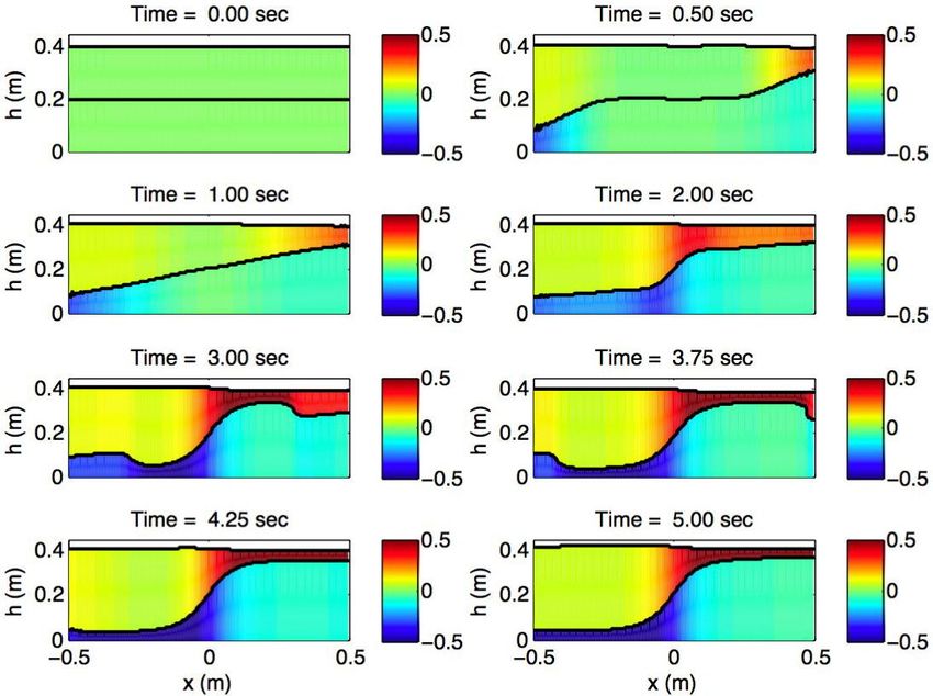
Abstract
                                                                                                              OSD
     Time-dependent, two layer hydraulic exchange flow is studied using an idealised shal-
     low water model. It is found that barotropic time-dependent perturbations, representing        3, 1999–2020, 2006
     tidal forcing, increase the baroclinic exchange flux above the steady hydraulic limit, with
 5   flux increasing monotonically with tidal amplitude (measured either by height or flux         Tides in exchange
     amplitude over a tidal period). Exchange flux also depends on the non-dimensional                    flows
     tidal period, γ, which was introduced by Helfrich (1995). Resonance complicates the
     relationship between exchange flux and height amplitude, but, when tidal strength is          L. M. Frankcombe and
     characterised by flux amplitude, exchange flux is a monotonic function of γ.                      A. McC. Hogg

10   1 Introduction                                                                                          Title Page

     Flow of stratified water through ocean straits makes an important contribution to the          Abstract        Introduction
     evolution of ocean stratification, affecting global circulation and the local dynamics of
                                                                                                   Conclusions      References
     estuaries and semi-enclosed basins. For example, exchange flow through the Strait
     of Gibraltar at the mouth of the Mediterranean Sea controls the salinity budget of the          Tables           Figures
15   evaporative Mediterranean basin (Bray et al., 1995). Furthermore, the dense, saline
     outflow of water from Gibraltar can be detected as a distinct water mass across the                J                  I
     North Atlantic (Sy, 1988; Harvey and Arhan, 1988). It follows that characterisation of
     flow through straits is an important problem, especially considering the difficulty most          J                   I

     ocean and climate models face in resolving strait dynamics.                                      Back                Close
20      Internal hydraulic theory can give a useful estimate of density-driven flow through
     straits in particular cases (Wood, 1970; Armi, 1986). This theory can be used to predict           Full Screen / Esc
     an upper bound for exchange flow through a strait (Armi and Farmer, 1987). However,
     this upper bound can be exceeded in cases where a time-dependent forcing, such as               Printer-friendly Version
     tidal flow, exists (Armi and Farmer, 1986).
                                                                                                      Interactive Discussion
25      Stigebrandt (1977) proposed a simple amendment to the hydraulic solution which
     showed reasonable agreement with laboratory experiments. This theory was super-
                                                                                                               EGU
                                               2000
seded by Armi and Farmer (1986), who formulated a quasi-steady solution based on
     hydraulically controlled solutions with a barotropic throughflow. The quasi-steady so-                    OSD
     lution assumed that tidal variations were sufficiently slow so that hydraulic control was
                                                                                                     3, 1999–2020, 2006
     continually established; however, hydraulic control itself is not well defined in a time de-
 5   pendent flow and it can be shown that tidal variations may exceed the frequency over
     which the quasi-steady solution is valid. Helfrich (1995) introduced a nondimensional          Tides in exchange
     parameter, γ, the ratio of tidal period to the time taken for a wave to traverse the strait.          flows
     It is defined as
             p                                                                                      L. M. Frankcombe and
           T g0 H                                                                                       A. McC. Hogg
     γ≡                                                                                       (1)
               l
10   where T is the period of the wave, g0 =g∆ρ/ρ is reduced gravity, H is the total fluid
     height and l is the length scale of the channel, i.e. the distance between the narrowest                 Title Page

     part of the channel (where channel width is b0 ) and the point where channel width is           Abstract        Introduction
     2b0 . Helfrich (1995) predicted that flux would depend upon both the dynamic strait
     length γ, and the amplitude of the tide. This prediction was consistent with simulations       Conclusions      References
15   from a simple numerical model with a rigid lid. Helfrich also conducted laboratory
                                                                                                      Tables           Figures
     experiments which showed that flux depends on γ, but that mixing and other effects
     act to reduce the flux.
                                                                                                         J                  I
         Additional experiments were conducted by Phu (2001) (reported by Ivey, 2004), in
     which both tidal amplitude and frequency were varied. It was found that exchange flux              J                   I
20   was strongly dependent on tidal amplitude, but that there was no systematic depen-
     dence upon tidal period, over a wide range of 2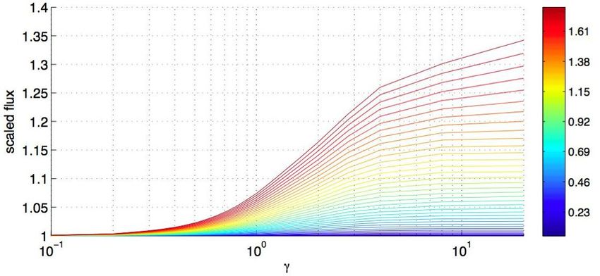
used a rigid lid). The waves modify the flux, which can be accurately measured, and
     the results are compared to the quasi-steady solution of Armi and Farmer (1986), the                   OSD
     predictions of Helfrich (1995) and the experimental results of Phu (2001).
                                                                                                  3, 1999–2020, 2006
        We begin the paper by outlining the model and boundary conditions in Sect. 2. Sec-
 5   tion 3 shows the results of the model, which are developed to span a wide parameter
     space in both the frequency and amplitude of time-dependent forcing. These results          Tides in exchange
     are discussed in Sect. 4, and application to geophysical flows is considered.                      flows

                                                                                                 L. M. Frankcombe and
     2 The Model                                                                                     A. McC. Hogg

     2.1 Shallow water equations
                                                                                                           Title Page
10   The model used here is formulated to include the physics of time-dependent exchange
     flows with the minimum possible alterations to the steady hydraulic equations. We            Abstract        Introduction
     therefore solve the one-dimensional nonlinear shallow water equations for flow along a
                                                                                                 Conclusions      References
     rectangular channel. The channel has length 2L and variable width b(x). We assume
     that flow occurs within two distinct immiscible fluid layers. The thickness of each layer     Tables           Figures
15   is hi (x, t) – as shown in Fig. 1. The layers are assumed to have constant density ρi ,
     and velocity ui (x, t) which depends upon horizontal, but not vertical, position.                J                  I
        The conservation of mass (or continuity) equation for each layer is given by
                                                                                                     J                   I
     ∂hi        1 ∂
           =−         (bui hi ) .                                                          (2)
      ∂t        b ∂x                                                                                Back                Close
     The conservation of momentum equations are
                                                                                                      Full Screen / Esc
     ∂u1      ∂u1      ∂                  ∂h2      ∂ 2 u1
20       + u1     = −g    (h2 + h1 ) + g0     + Ah                                         (3)
     ∂t       ∂x       ∂x                 ∂x       ∂x 2                                            Printer-friendly Version

     and                                                                                            Interactive Discussion
     ∂u2      ∂u2      ∂                ∂ 2 u2
         + u2     = −g   (h + h1 ) + Ah        ,                                           (4)
     ∂t       ∂x       ∂x 2             ∂x 2                                                                 EGU
                                            2002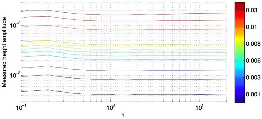
0
where the reduced gravity, g , is defined as follows:
g(ρ1 − ρ2 )
OSD
g0 ≡ .
ρ1 3, 1999–2020, 2006
Note that we have included a lateral viscosity with a constant coefficient Ah , which is
required for numerical stability but is minimised in the simulations. Tides in exchange
5 The solution of (2)–(4) under the assumption of a steady flow may yield hydrauli- flows
cally controlled flow solutions (depending upon the boundary conditions at either end
L. M. Frankcombe and
of the channel). The full time-dependent equations may be solved numerically in a
A. McC. Hogg
straightforward manner; but results are again dependent upon the correct boundary
conditions.
Title Page
10 2.2 Boundary conditions
Abstract Introduction
The boundary conditions used for this model are the characteristic open boundary
conditions based on the time-integrating conditions proposed by Nycander and Döös Conclusions References
(2003) and further developed for inertial flows by Nycander et al. (2006). These con-
± ± Tables Figures
ditions require us to specify characteristic variables aE and aI at each of the open
15 boundaries. The variables are defined as
" # J I
1 H u + H u
a±
1 1 2 2
E
= h1 + h2 ± , (5) J I
2H
p
gH
Back Close
s
1 H h − H2 h1 H1 H2
a± = 1 2 ± (u2 − u1 ) . (6) Full Screen / Esc
I 2H H g0 H − ∆U 2
Printer-friendly Version
These equations are formulated by linearising the equations about a state with layer
heights H1 and H2 (where H=H1 + H2 ), and velocity difference ∆U between the layers. Interactive Discussion
EGU
2003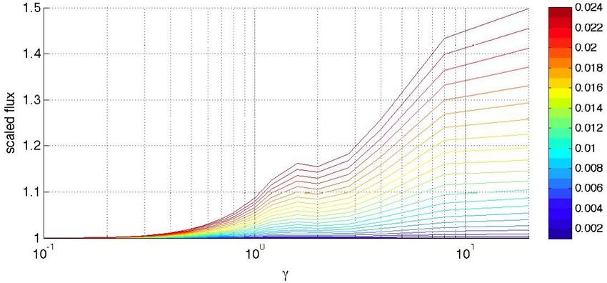
The conditions are implemented as follows. Assume, for example, that the boundary
     is an h-point of a staggered grid. Then we must specify the inward travelling charac-
                         ±      ±
                                                                                                               OSD
     teristic variables aE and aI . Having done that, the values of h1 and h2 at the boundary
                                                                                                     3, 1999–2020, 2006
     can be expressed in terms of a± E
                                       , a±
                                          I
                                            and the values of u1 and u2 at the point just inside:
                                        H1 H1 u1 + H2 u2
 5   h1 (∓L) = 2H1 a±
                    E
                      − 2Ha±
                           I
                             ∓                                                                      Tides in exchange
                                        H
                                               p
                                                 gH                                                        flows
                             s
                                    H1 H2                                                           L. M. Frankcombe and
                         ±                       (u1 − u2 ),                                  (7)
                                 g0 H   − ∆U 2                                                          A. McC. Hogg

                                        H2 H1 u1 + H2 u2
     h2 (∓L) = 2H2 a±
                    E
                      + 2Ha±
                           I
                             ∓
                                        H
                                               p                                                              Title Page
                                                 gH
                             s
                                    H1 H2                                                            Abstract        Introduction
                         ∓                       (u1 − u2 ).                                  (8)
                                 g0 H − ∆U 2                                                        Conclusions      References

10      The above conditions are suitable for sub-critical flow, but this model also needs to         Tables           Figures
     be able to simulate supercritical two-layer flow. The model is designed to switch to
     supercritical flow boundary conditions subject to a test on the criticality of the flow.
                                                                                                         J                  I
     There are two modes of supercritical flow (i.e. supercritical with respect to barotropic
     and baroclinic modes) and therefore two tests. The test for supercritical barotropic flow          J                   I
15   is based on the linear phase speed of a barotropic wave. When
                                                                                                       Back                Close
     h1 u1 + h2 u2 q
                   > g(h1 + h2 ),                                                           (9)
        h1 + h2                                                                                          Full Screen / Esc

     at the right hand end of the channel, flow is adjudged supercritical. There is an anal-
                                                                                                      Printer-friendly Version
     ogous condition at the left hand end of the channel. When this test is satisfied, the
     supercritical open boundary conditions are simply                                                 Interactive Discussion
     ∂h1   ∂h2
20       =     = 0,                                                                         (10)
     ∂x    ∂x                                                                                                   EGU
                                                        2004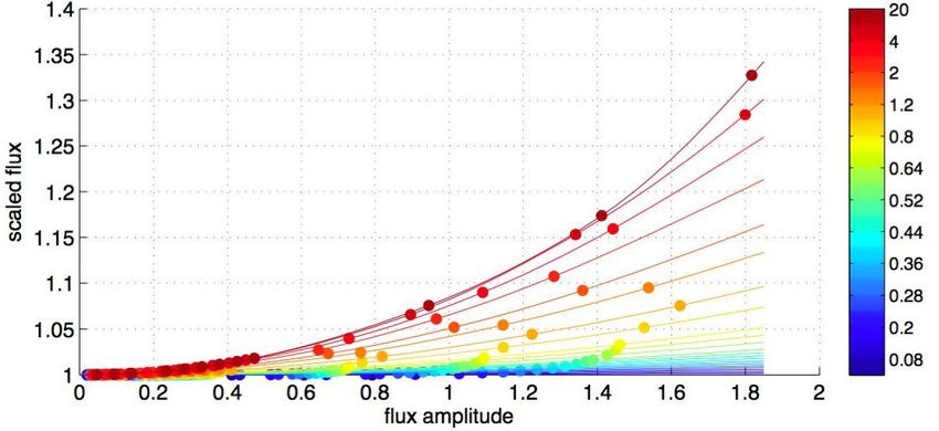
which replaces (7)-(8).
       Internally supercritical flow is more complicated. Firstly, using linear internal                        OSD
     wavespeeds to test for internal criticality, we obtain
                     s                                                                                3, 1999–2020, 2006
     h2 u1 + h1 u2        h1 h2
                                   g0(h1 + h2 ) − (u1 − u2 )2 ,

                   >                                                                (11)
        h1 + h2        (h1 + h2 )2                                                                   Tides in exchange
                                                                                                            flows
 5   at the right hand end of the channel (and an analogous condition for the left hand end).
     It should be noted that the RHS of this condition becomes imaginary when shear is               L. M. Frankcombe and
     strong, in which case the wavespeeds coalesce and waves are unstable. Therefore,                    A. McC. Hogg
     we propose that a suitable test for criticality is simply
                      s
     h2 u1 + h1 u2         h1 h2                                                                               Title Page
                    >               Θ,                                                   (12)
        h1 + h2         (h1 + h2 )2
                                                                                                      Abstract        Introduction
10   where
                                                                                                 Conclusions      References
     Θ ≡ max 0, g0(h1 + h2 ) − (u1 − u2 )2 .                                                 (13)
                                                                                                       Tables           Figures
       The boundary conditions for internally supercritical flow are found by assuming that
     the internal mode is captured primarily by interfacial height, and so we set                         J                  I

     ∂h1                                                                                                 J                   I
         = 0,                                                                                (14)
     ∂x
                                                                                                        Back                Close
15   with h2 calculated using the addition of (7) and (8).
                                                                                                          Full Screen / Esc
     2.3 Numerical implementation
                                                                                                       Printer-friendly Version
     The domain is spatially discretised on a staggered grid. Velocity is calculated at the
     faces of the cells, while layer height is calculated at the centre of the cell. The equations      Interactive Discussion
     may then be integrated in time using centred differences. The staggered grid is defined
20   so that the near-boundary values of velocity can be explicitly calculated from (3,4).                       EGU
                                                  2005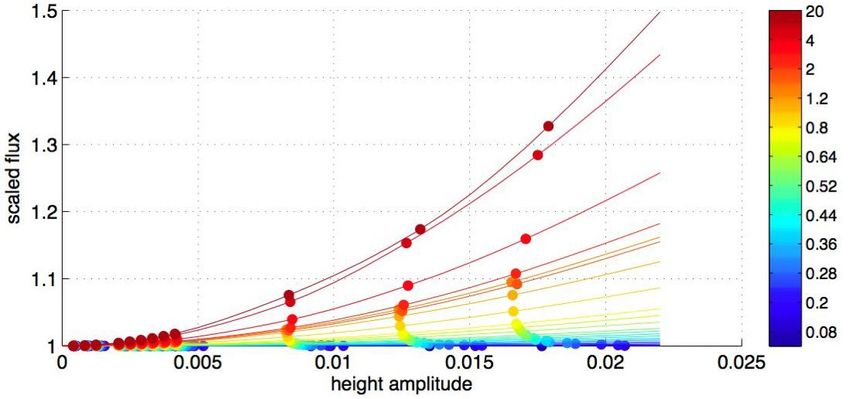
The temporal discretisation employs a leapfrog timestep scheme. Leapfrog timestep-
ping routines can produce two diverging solutions. To eliminate this potential problem, OSD
data from different time levels are mixed every 1000 timesteps. The standard parame-
3, 1999–2020, 2006
ter set for the simulations is shown in Table 1.
Tides in exchange
5 3 Results flows
3.1 Exchange flows L. M. Frankcombe and
A. McC. Hogg
The model is initialised with two constant depth, zero velocity layers. Layer depth vari-
ations and velocity are induced by specifying the characteristic boundary conditions,
as seen in the series of snapshots in Fig. 2, which shows the development of the ex- Title Page
10 change flow. Internal waves propagate from either side of the domain, reaching the
centre of the constriction after about 1 s. Over the next second, hydraulic control is Abstract Introduction
established at the centre of the channel, and features resembling hydraulic jumps are
Conclusions References
formed. It should be noted that the model equations used here cannot resolve shocks
of this nature, and these jump-like features are only stabilised with viscosity. These Tables Figures
15 features propagate out of the domain, leaving a final steady state exactly matching the
two-layer maximal hydraulic exchange flow solution, in which flow is internally super- J I
critical at both ends of the channel. It is notable that there are no significant reflections
from the characteristic open boundary conditions during this adjustment process – this J I
issue is examined more closely by Nycander et al. (2006). Back Close
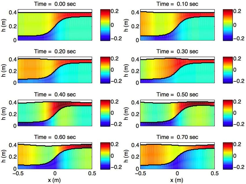
20 Time dependence is introduced to this flow by sinusoidally varying the left boundary
+
condition coefficient, ae , with a period of 0.5 s. This simulates a barotropic wave en- Full Screen / Esc
tering from the left, as seen in Fig. 3. The incoming wave travels towards the centre of
the channel where it interacts with the contraction, causing reflections (both baroclinic Printer-friendly Version
and barotropic) to travel back to the left, while the original barotropic wave, which now
Interactive Discussion
25 includes a small baroclinic component, continues to the right. The waves steepen due
to nonlinearity as they propagate along the channel.
EGU
2006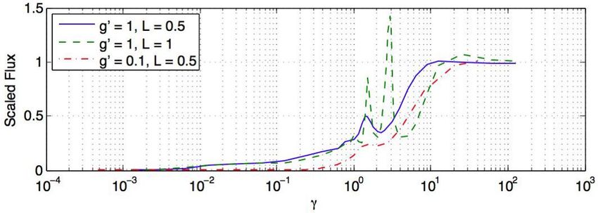
Barotropic flux as a function of time at the left-hand boundary is shown in Fig. 4.
     Note that the system takes several periods for the oscillations to become regular, as                   OSD
     instantaneous flux is modulated by waves reflected off the contraction. For this rea-
                                                                                                   3, 1999–2020, 2006
     son all results in the following sections were calculated after the initial adjustment had
 5   occurred.
                                                                                                  Tides in exchange
     3.2 Exchange flux in time-dependent systems                                                         flows

     The quantity of primary interest in these simulations is the flux of volume (or mass)        L. M. Frankcombe and
     exchanged. We quantify this by calculating the total flux in each layer as a function of         A. McC. Hogg
     time, integrating over a tidal period and averaging the (absolute value of the) two layer
10   fluxes. This baroclinic exchange flux is then proportional to the net exchange of mass
     (or passive tracer) through the channel. Figure 5 shows the exchange flux anomaly                      Title Page
     as a function of nondimensional period γ, for several cases. The flux anomaly has
                                                                                                   Abstract        Introduction
     been scaled by the quasi-steady flux, which was calculated numerically from a series
     of steady simulations and sets a theoretical upper limit for the flux.                       Conclusions      References
15      In the small period (small γ) limit the flux anomaly approaches zero (the steady
                                                                                                    Tables           Figures
     hydraulic limit), and in the large γ limit it approaches the quasi-steady solution in each
     of the three cases shown. This is consistent with the predictions of Helfrich (1995);
     however here the flux is not a monotonically increasing function of γ. Instead, there             J                  I

     are additional local maxima (the largest being at γ≈3) which sometimes exceed the                J                   I
20   quasi-steady limit. These discrepancies are greatest when g0 is large, and when the
     domain length L is increased (dashed line in Fig. 5).                                           Back                Close
        These peaks are due to resonance in the channel between the open boundary and
                                                                                                       Full Screen / Esc
     the contraction. Although the resonance is damped it is continually forced by incoming
     energy, and thus has a bounded amplitude. Resonance is strongest when the channel
                                                                                                    Printer-friendly Version
25   is long (allowing time for nonlinear steepening to occur), and can be minimised using
             0
     small g (possibly because interactions between barotropic and baroclinic modes are              Interactive Discussion
     minimised in this case). The resonant period depends on the channel length L as
     expected. This resonance occurs even though reflections caused by the boundary
                                                                                                              EGU
                                                   2007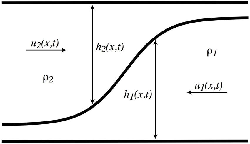
conditions are significantly smaller than other schemes (Nycander et al., 2006), so it
     follows that simulations with other boundary conditions, or lab experiments with solid                 OSD
     end walls, will experience greater problems with resonance. We do not investigate
                                                                                                  3, 1999–2020, 2006
     the source of resonance in this paper; instead, for all tests below, the simulations use
 5   L=0.5 and g0 =0.1 to minimise the effect. We use these simulations to quantify the
     effect of tidal period and amplitude on exchange flux.                                      Tides in exchange
                                                                                                        flows
     3.3 Rescaling amplitude
                                                                                                 L. M. Frankcombe and
     Although resonance is minimised through choice of parameters, it cannot be entirely             A. McC. Hogg
     eliminated. Notably, this resonance was not observed in Helfrich’s (1995) simulations
10   (which used a rigid upper surface and imposed barotropic fluctuations at the contrac-
     tion). For consistency with previous work, we prefer to further reduce resonant effects               Title Page
     by taking the observed amplitude of the waves at the centre of the channel (instead
                                                                                                  Abstract        Introduction
     of the amplitude originally imposed at the boundary). It is then possible to define two
     tidal amplitudes. Firstly, a represents the peak-to-trough amplitude of fluid height over   Conclusions      References
15   the tidal cycle. We refer to this as the height amplitude and it is analogous to the
                                                                                                   Tables           Figures
     method used by Phu (2001) to characterise tidal amplitude. Secondly we can use the
     barotropic flux amplitude, Helfrich’s qb0 parameter, which is defined as
                                                                                                      J                  I
             ub0
     qb0   ≡p                                                                            (15)
                                                                                                     J                   I
              g0 H
     where ub0 is the peak-to-trough amplitude of barotropic velocity at the throat over the        Back                Close

20   tidal cycle.                                                                                     Full Screen / Esc
        This allows us to plot measured (a) height and (b) flux amplitude against γ, as in
     Fig. 6 (note the logarithmic axes). Here we see the effect of the resonance – the
     measured amplitude, for a given value of imposed a+
                                                                                                   Printer-friendly Version
                                                          e amplitude, is not independent of
     γ. Moreover, the two measures of amplitude differ significantly as a function of γ.            Interactive Discussion
                                                                +
25      Numerous simulations across a large range in γ and ae amplitude were conducted
     and the results have been interpolated onto lines of (a) constant height amplitude, and                 EGU
                                             2008
(b) constant flux amplitude. We can now plot flux as a function of γ for a number of
different cases – see Fig. 7. Figure 7a shows a peak at γ=1.5, indicating that height OSD
amplitude is not a good measure of the tidal effect on exchange flows. It follows that
3, 1999–2020, 2006
for cases with greater amplitude and stronger stratification, such as the dashed lines in
5 Fig. 5, the height amplitude will be a very poor descriptor of the tidal effects. Figure 7b,
on the other hand, clearly shows a smooth monotonic transition of flux with γ when Tides in exchange
flux amplitude is used as the metric. These results are consistent with predictions of flows
Helfrich (1995). Thus flux amplitude would appear to be a more useful metric than
L. M. Frankcombe and
height amplitude.
A. McC. Hogg
10 The results are re-plotted in Fig. 8, showing amplitude vs flux for each of the above
cases. The panels, showing scaled flux as a function of height and flux amplitude
respectively, both show a clear tendency for flux to increase with amplitude. This is
Title Page
consistent with expectations and with results of Phu (2001). The differences between
the height and flux amplitude are once again noticeable, however the overall trend Abstract Introduction
15 remains the same in both cases.
Conclusions References
Tables Figures
4 Discussion and conclusions
The results of these simulations confirm that time-dependent forcing leads to an in- J I
crease in exchange flux compared to the steady state case. Tidal amplitude, as mea-
J I
sured by either height or flux amplitude, has a strong effect on flux, with flux increasing
20 monotonically with amplitude. Back Close
Flux also depends on the nondimensional tidal period γ. However, resonance with
Full Screen / Esc
the open boundary conditions in the numerical simulations performed here modulates
the response. Resonance produces effects which depend strongly upon tidal period.
Nevertheless, if one uses the flux amplitude to characterise tidal strength, then the ex- Printer-friendly Version
25 change flux is a monotonic function of γ. The relationship between exchange flux and Interactive Discussion
height amplitude, on the other hand, is more complicated. Depending on the strength
of resonance this may result in a non-monotonic relationship between exchange flux
EGU
2009and γ (when a is held constant).
These observations may explain some outstanding discrepancies between previous OSD
studies on this topic. Phu (2001) (reported by Ivey, 2004) used the height amplitude
3, 1999–2020, 2006
to characterise tidal strength and found no systematic dependence upon γ over a wide
5 range in parameter space, while Helfrich (1995) found a strong dependence of flux
amplitude on γ. Reflections from the solid tank walls in Phu’s (2001) experiments Tides in exchange
would have produced resonance, especially for large values of γ (long periods) where flows
there is ample time for reflections to travel from the walls of the tank to the contraction.
L. M. Frankcombe and
Thus, the height amplitude formalism used by Phu (2001) to characterise tidal strength
A. McC. Hogg
10 may be distorted by resonant effects.
It follows from this analysis that one can most easily describe geophysical obser-
vations using barotropic flux amplitude. However, measurements of tidal range are
Title Page
easiest to quantify in terms of height amplitude, rather than flux. It is likely that a
barotropic model of the tidal velocities will be required to be able to apply Helfrich’s Abstract Introduction
15 (1995) formalism with any confidence.
Conclusions References
Acknowledgements. J. Nycander contributed significantly to this work, in assisting with the
implementation of the boundary conditions and commenting on early drafts of this manuscript. Tables Figures
LMF was funded by an A. L. Hales Scholarship, and AMH acknowledges the support of an
Australian Research Council Postdoctoral Fellowship (DP0449851). This work was supported J I
20 by the National Facility of the Australian Partnership for Advanced Computing.
J I
References Back Close
Full Screen / Esc
Armi, L.: The hydraulics of two flowing layers with different densities, J. Fluid Mech., 163,
27–58, 1986. 2000
Armi, L. and Farmer, D. M.: Maximal two-layer exchange through a contraction with barotropic Printer-friendly Version
25 net flow, J. Fluid Mech., 164, 27–51, 1986. 2000, 2001, 2002
Armi, L. and Farmer, D. M.: A Generalization of the concept of Maximal Exchange in a Strait, Interactive Discussion
J. Geophys. Res., 92, 14 679–14 680, 1987. 2000
EGU
2010Bray, N., Ochoa, W. J., and Kinder, T.: The role of the interface in exchange through the Strait
of Gibraltar, J. Geophys. Res., 100, 10 755–10 776, 1995. 2000 OSD
Harvey, J. and Arhan, M.: The Water Masses of the Central North Atlantic in 1983-84, J. Phys.
Oceanogr., 18, 1855–1875, 1988. 2000 3, 1999–2020, 2006
5 Helfrich, K. L.: Time-dependent two-layer hydraulic exchange flow, J. Phys. Oceanogr., 25,
359–373, 1995. 2000, 2001, 2002, 2007, 2008, 2009, 2010
Ivey, G. N.: Stratification and mixing in sea straits, Deep-Sea Res. II, 51, 441–453, 2004. 2001, Tides in exchange
2010 flows
Nycander, J. and Döös, K.: Open boundary conditions for barotropic waves, J. Geophys. Res.,
10 108, 10.1029/2002JC001 529, 2003. 2003 L. M. Frankcombe and
Nycander, J., Hogg, A. M., and Frankcombe, L. M.: Open boundary conditions for nonlinear A. McC. Hogg
shallow water models, Ocean Modell., p. Submitted for Review, 2006. 2003, 2006, 2008,
2012
Phu, A.: Tidally forced exchange flows, Honours thesis, University of Western Australia, 2001. Title Page
15 2001, 2002, 2008, 2009, 2010
Stigebrandt, A.: On the effects of barotropic current fluctuations on the two-layer transport Abstract Introduction
capacity of a constriction, J. Phys. Oceanogr., 7, 118–122, 1977. 2000
Sy, A.: Investigation of large-scale circulation patterns in the Central North Atlantic: the North Conclusions References
Atlantic Current, the Azores Current, and the Mediterranean Water plume in the area of the
Tables Figures
20 Mid-Atlantic Ridge, Deep Sea Res., 35, 383–413, 1988. 2000
Wood, I. R.: A lock exchange flow, J. Fluid Mech., 42, 671–687, 1970. 2000
J I
J I
Back Close
Full Screen / Esc
Printer-friendly Version
Interactive Discussion
EGU
2011OSD
3, 1999–2020, 2006
Tides in exchange
flows
Table 1. Standard physical and computational parameters for simulations. See Nycander et al.
(2006) for an explanation for the values of the internal and external characteristics. L. M. Frankcombe and
Parameter Value Description A. McC. Hogg
l 0.5 m Constriction length
Ah 0.008 m2 /s Horizontal viscosity
Title Page
H 0.4 m Total fluid height
bmin 0.1 m Minimum channel width (at x = 0) Abstract Introduction
bmax 0.2 m Maximum channel width (at x = ±L)
2
g0 0.1 m/s Reduced gravity Conclusions References
L 0.5 m Channel length Tables Figures
−7
∆t 3×10 s Timestep
n 201 Number of gridpoints
J I
∆x 0.005 m Gridlength
+
ae 0.017 External BC coefficient at LHS J I
a−e 0.0 External BC coefficient at RHS
a+i 0.07028 Internal BC coefficient at LHS Back Close
−
ai –0.07028 Internal BC coefficient at RHS
Full Screen / Esc
Printer-friendly Version
Interactive Discussion
EGU
2012OSD
3, 1999–2020, 2006
Tides in exchange
flows
L. M. Frankcombe and
A. McC. Hogg
Title Page
(a) Abstract Introduction
Conclusions References
Tables Figures
J I
J I
Back Close
center (b) Full Screen / Esc
Fig. 1. Schematic showing (a) plan and (b) elevation view of the flow.
Printer-friendly Version
Interactive Discussion
EGU
2013OSD
3, 1999–2020, 2006
Tides in exchange
flows
L. M. Frankcombe and
A. McC. Hogg
Title Page
Abstract Introduction
Conclusions References
Tables Figures
J I
J I
Back Close
Full Screen / Esc
Fig. 2. Development of two layer flow (for a channel with bmax =0.3 m).
Printer-friendly Version
Interactive Discussion
EGU
2014OSD
3, 1999–2020, 2006
Tides in exchange
flows
L. M. Frankcombe and
A. McC. Hogg
Title Page
Abstract Introduction
Conclusions References
Tables Figures
J I
J I
Back Close
Full Screen / Esc
Fig. 3. Propagation of a wave through the channel.
Printer-friendly Version
Interactive Discussion
EGU
2015OSD
3, 1999–2020, 2006
Tides in exchange
flows
L. M. Frankcombe and
A. McC. Hogg
Title Page
Abstract Introduction
Conclusions References
Tables Figures
J I
Fig. 4. Barotropic flux measured at the left hand boundary.
J I
Back Close
Full Screen / Esc
Printer-friendly Version
Interactive Discussion
EGU
2016OSD
3, 1999–2020, 2006
Tides in exchange
flows
L. M. Frankcombe and
A. McC. Hogg
Title Page
Abstract Introduction
Conclusions References
Tables Figures
J I
Fig. 5. Flux anomaly with different values of g0 and L, scaled by the quasi-steady flux.
J I
Back Close
Full Screen / Esc
Printer-friendly Version
Interactive Discussion
EGU
2017OSD
3, 1999–2020, 2006
Tides in exchange
flows
L. M. Frankcombe and
A. McC. Hogg
Title Page
(a)
Abstract Introduction
Conclusions References
Tables Figures
J I
J I
Back Close
(b)
Full Screen / Esc
Fig. 6. Observed (a) height and (b) flux amplitudes are plotted against γ for different imposed
a+e amplitudes.
Printer-friendly Version
Interactive Discussion
EGU
2018OSD
3, 1999–2020, 2006
Tides in exchange
flows
L. M. Frankcombe and
A. McC. Hogg
Title Page
(a)
Abstract Introduction
Conclusions References
Tables Figures
J I
J I
Back Close
(b)
Full Screen / Esc
Fig. 7. Flux is plotted against γ with (a) measured height amplitude and (b) measured flux
amplitude in colour.
Printer-friendly Version
Interactive Discussion
EGU
2019OSD
3, 1999–2020, 2006
Tides in exchange
flows
L. M. Frankcombe and
A. McC. Hogg
Title Page
(a)
Abstract Introduction
Conclusions References
Tables Figures
J I
J I
(b) Back Close
Fig. 8. Flux is plotted against (a) measured height amplitude and (b) measured flux amplitude, Full Screen / Esc
with γ in colour. Solid circles show the original points from which the other points have been
interpolated. Printer-friendly Version
Interactive Discussion
EGU
2020You can also read