Towards B-Spline Atomic Structure Calculations - MDPI
←
→
Page content transcription
If your browser does not render page correctly, please read the page content below
atoms
Article
Towards B-Spline Atomic Structure Calculations
Charlotte Froese Fischer

                                          Department of Computer Science, University of British Columbia, Vancouver, BC V6T1Z4, Canada; cff@cs.ubc.ca

                                          Abstract: The paper reviews the history of B-spline methods for atomic structure calculations for
                                          bound states. It highlights various aspects of the variational method, particularly with regard to the
                                          orthogonality requirements, the iterative self-consistent method, the eigenvalue problem, and the
                                          related SPHF, DBSR - HF, and SPMCHF programs. B-splines facilitate the mapping of solutions from one
                                          grid to another. The following paper describes a two-stage approach where the goal of the first stage
                                          is to determine parameters of the problem, such as the range and approximate values of the orbitals,
                                          after which the level of accuracy is raised. Once convergence has been achieved the Virial Theorem,
                                          which is evaluated as a check for accuracy. For exact solutions, the V/T ratio for a non-relativistic
                                          calculation is −2.

                                          Keywords: atomic structure; B-splines; eigenvalue methods; Newton–Raphson method; variational theory

                                          1. Introduction
                                                In 1996 Oleg Zatsarinny published a program for computing matrix elements in a
                                non-orthogonal radial basis in which configuration state functions (CSFs) were expanded in
                                   determinants [1]. A non-orthogonal basis can greatly reduce the size of multiconfiguration
Citation: Fischer, C.F. Towards           wave function expansions. The orthogonal versus non-orthogonal issue is a complex one,
B-Spline Atomic Structure                 so I invited Oleg for a three-month visit, with the National Science Foundation support
Calculations. Atoms 2021, 9, 50.          for members of the former Soviet Union. Before he left, I shared with him the B-spline
https://doi.org/10.3390/atoms             library I had developed for calculations of high accuracy “good to the last bit”. Oleg
9030050                                   improved and extended the library, which became the basis for the BSR code he published
                                          in 2006 [2] for both non-relativistic and the Breit–Pauli R-matrix theory. It was not until
Academic Editor: Ulrich D.                2011 [3] that I published a non-relativistic B-spline Hartree-Fock program for bound states
Jentschura
                                          using the extended library. In the mean time, Oleg extended BSR to Dirac relativistic theory
                                          where the R-matrix approach relies on eigenvectors of a B-spline matrix at the boundary.
Received: 13 July 2021
                                          However with the traditional Galerkin method applied to the pair of first-order differential
Accepted: 27 July 2021
                                          equations, spurious solutions appeared for the R-matrix.
Published: 31 July 2021
                                                The presence of spurious solutions from the application of the Galerkin methods is
                                          well known—a Google search for “Galerkin spurious” has 165,000 responses from areas
Publisher’s Note: MDPI stays neutral
                                          of theoretical physics, applied mathematics, and engineering. Inspired by the work of
with regard to jurisdictional claims in
                                          Igarashi [4,5], I had the idea that the problem was related to the fact that Dirac equations
published maps and institutional affil-
iations.
                                          are a system of first-order equations. I showed that the problem also occurs for y00 = −λ2 y,
                                          with boundary conditions y(0) = 0 and y( R) = 0, when the single second-order equation
                                          is replaced by a pair of first-order equations. Igarashi was focusing mostly on kinetically-
                                          balanced basis sets but tried also some other ideas like using B-splines of a different
                                          order. If we think of the Galerkin method approximating the small component by say,
Copyright: © 2021 by the author.
                                          Qks (r ) = ∑i ci Biks (r ), where Biks (r ) is a B-spline of order k s (or piecewise polynomial of
Licensee MDPI, Basel, Switzerland.
This article is an open access article
                                          degree k s − 1), then the large component is proportional to (d/dr − κ/r ) Qk (r ), namely
distributed under the terms and           piecewise polynomials of degree k s − 2 with a B-spline basis of order k s − 1. Representing
conditions of the Creative Commons        these functions by a higher-order polynomial presents difficulties that would not arise if
Attribution (CC BY) license (https://     a lower order of splines were used. In my test case, the eigenvalues from using different
creativecommons.org/licenses/by/          orders for pairs of equations were the same as those from a single second-order equation,
4.0/).                                    indicating that the problem was not just a Dirac equation-related problem. Splines of

Atoms 2021, 9, 50. https://doi.org/10.3390/atoms9030050                                                      https://www.mdpi.com/journal/atoms
Atoms 2021, 9, 50 2 of 14
different orders worked beautifully for the R-matrix approach as well as the Thomas–
Reiche–Kuhn sum rule and all our other tests. I convinced Oleg that we should prepare
a paper for Physical Review Letters, but the referee was not as excited by this result as I
was. Oleg was not prepared to argue so the paper was published in Computer Physics
Communication [6].
The present paper is dedicated to the memory of Oleg Zatsarinny who extended the
bound state B-spline codes to the fully relativistic DBSR - HF version [7].
2. In the Beginning ...
In the early days of computing, atomic and molecular calculations relied either on
finite-difference methods based on numerical procedures developed by Hartree [8], or an-
alytic methods based on basis sets such as Slater-type orbitals [9]. Bachau et al. [10] in
their excellent review on B-splines, refer to these methods as local versus global methods,
respectively, in that finite difference methods relied on only a few values at adjacent points
of a grid in specifying an approximation. Much changed when de Boor [11] published his
book in 1985 about B-splines with a local but complete basis for piece-wise polynomial
approximations along with Fortran programs for standard spline procedures. Among the
first to use his codes were Johnson and Sapirstein [12], who used B-splines to generate
their numerical basis set for perturbation theory that greatly advanced the theory. How-
ever B-splines also offer advantages for a wide range of applications as Bachau et al., show
in their extensive review.
By the 1990s, the non-relativistic Hartree–Fock variational method had evolved into a
multiconfiguration theory as implemented in the MCHF 77 [13] program. Later this theory
was extended to include relativistic corrections through a Breit–Pauli approximation and,
together with programs for atomic properties (hyperfine, isotope shifts, and transition
probabilities), became an atomic structure package ATSP 2K [14]. All calculations were
based on numerical procedures and supported a limited amount of non-orthogonality of
the radial basis [15] of one or at most two overlap integrals.
With the development of faster computers along with considerable more memory,
an interesting question arose—what is the best method for solving the MCHF equations? The
latter required node counting to control the convergence of an integro-differential equation
with many solutions, dealing also with Lagrange multipliers for satisfying orthonormality.
This paper reviews the development of spline methods for variational approaches to
solutions of the wave equation for atoms with the assumption that the reader is familiar
with the basic properties of splines as presented by Bachau et al. [10]. Unlike the latter,
the emphasis here is more on the computational methods and the programs that have
emerged rather than their application.
3. The B-Spline Basics
A spline approximation of order k s is an approximation that is a piecewise polynomial
of degree k s − 1 (with k s coefficients) in intervals defined by “knots” that define a grid.
In applications, the grid itself, in a sense, is arbitrary but the choice of grid can have a large
influence on the accuracy of an approximation.
3.1. Spline Grid for Radial Functions
In atomic structure applications, it is convenient to define the grid in terms of the
variable t = Zr (the hydrogenic case) and then transform to the current value of Z. Let
h = 1/2m . This is not strictly necessary, but it ensures that the arithmetic is exact in binary
arithmetic. Then:Atoms 2021, 9, 50 3 of 14
ti = 0 for i = 1, . . . , k s (1)
t i = t i −1 + h for i = k s + 1, . . . , k s + m (2)
t i = t i −1 (1 + h ) for i = k s + m + 1, . . . , ns + 1 (3)
ti = t ns + 1 for i = ns + 2, . . . , ns + k s (4)
ri = ti /Z for i = 1, ns + k s (5)
Thus the grid is linear for m intervals near the origin after the t = 0 knots of multiplicity
k s , then linear in log(r ). If continuum calculations are involved, the range may be extended
to include equally-spaced values at the end of the exponential range, followed by final
knots of t = tmax of multiplicity k s . The above grid is most appropriate for a finite nucleus.
The number of non-zero intervals between knots is ns − k s + 1 where ns is the number
of basis states. Note also that, the end of the exponential region, t = tns +1 defines the
maximum range R of the bound-state orbitals, that are assumed to be zero for r > R.
In an early B-spline study, Froese Fischer and Parpia [16] studied the accuracy of the
application of B-splines to the Dirac equation for He with a grid over the range (0, 40),
comparing a grid for ρ = r1/4 with a grid for ρ = log(r ). The former was considerably
more accurate but is rarely used other than for plotting since r = 0 transforms to ρ = 0 in
the first transformation, whereas in the latter it transforms to −∞. However, an advantage
of splines is that points need not be equally spaced so r = 0 can be chosen as a grid-point
(as in Equation (1)) even when the remaining grid-points are on an exponential grid.
3.2. Integration Methods
The piecewise polynomial values are represented by k s values at the Gaussian points
for Gauss–Legendre integration. Then,
Z 1 ks
0
f ( x )dx = ∑ gw ( x i ) f ( x i ), (6)
i =1
where gw ( xi ) are the Gaussian weights at the Gaussian points xi . This formula is exact for
integrands f ( x ) that are polynomials of degree 2k s − 1.
3.3. Slater Integrals
A detailed analysis of algorithms for the calculation of Slater integrals was reported
by Qiu and Froese Fischer [17], and will be summarized here.
Let a, b, c, d denote a set of nl quantum numbers associated with a radial function:
P( a; r ) = ∑ ai Bi (r) (7)
i
with similar expansions for b, c, and d. Then,
Rk ( a, b; c, d) = ∑ ∑ ∑0 ∑0 ai bj ci0 d j0 Rk (i, j; i0 , j0 ), (8)
i j i j
where,
Z RZ R k
r<
Rk (i, j; i0 , j0 ) = B (r ) Bj (r2 ) Bi0 (r1 ) Bj0 (r2 )dr1 dr2
k +1 i 1
(9)
0 0 r>
will be referred to as B-spline Slater integrals. Many symmetries exist. Furthermore,
Rk (i, j; i0 , j0 ) = 0 if |i − i0 | > k s , or
= 0 if | j − j0 | > k s . (10)
Symmetry and the “local” property of these integrals, greatly reduce the number of
B-spline Slater integrals included in the summation.Atoms 2021, 9, 50 4 of 14
The spline-approximation divides the integration range into sub-intervals and the
two-dimensional integration into patches or “cells”. Thus the fundamental process is one
of integration over a cell, riv ≤ r1 ≤ riv +1 and r jv ≤ r2 ≤ riv +1 , namely,
jv + 1 r k
Z r Z r
i v +1
<
B (r ) Bj (r2 ) Bi0 (r1 ) Bj0 (r2 )dr1 dr2 .
k +1 i 1
(11)
riv r jv r>
However for an off-diagonal cell, the above two-dimensional integral is separable and
equal to (for iv < jv ):
Z r Z r
i v +1 jv +1
Bi (r1 )r1k Bi0 (r1 )dr1 Bj (r2 )(1/r2k+1 ) Bj0 (r2 )dr2
riv r jv
≡ r k (i, i0 ; iv ) × r −(k+1) ( j, j0 ; jv ), (12)
where r k (i, i0 ; iv ) and r −(k+1) ( j, j0 ; jv ) are referred to as moments.
The diagonal cells reduce to integrations over upper and lower triangles or, through
an interchange of arguments, as:
Rk (i, j; i0 , j0 ; iv ) = Rk∆ (i, j; i0 , j0 ; iv ) + Rk∆ ( j, i; j0 , i0 ; iv ) (13)
and Z r Z r
i v +1 1 1
Rk∆ (i, j; i0 , j0 ; iv ) = B (r ) B 0 (r )dr1
k +1 i 1 i 1
r2k Bj (r2 ) Bj0 (r2 )dr2 . (14)
riv r1 riv
Thus the computational complexity of an integration over a diagonal cell is O(k2s ) and
for the Rk (i, j; i0 , j0 ) array, it is O(ns k2s ). Furthermore, when all B-splines are defined on an
exponential grid where ti+1 = (1 + h)ti , (as in the middle region of the logarithmic grid)
scaling laws can be applied, namely:
h Bi+1 (r )|r k | Bj+1 (r )i = (1 + h)1+k h Bi (r )|r k | Bj (r )i
h Bi+1 (r )|1/r k+1 | Bj+1 (r )i = (1 + h)−k h Bi (r )|1/r k+1 | Bj (r )i
Rk (i + 1, j + 1; i0 + 1, j0 + 1) = (1 + h) Rk (i, j; i0 , j0 ). (15)
With such a grid, some Slater integrals would be computed using the basic integration
procedures and others could be scaled.
4. Tensor Products of B-Splines as a Basis
Traditionally, the wave functions for multi-electron systems are expanded in terms
of configuration state functions (CSFs) that are products of one-electron wave functions
(or orbitals) where, for bound-state problems, the latter provides an orthonormal basis.
An early spline study of the 1s2 , 1s2s 1 S or 3 S, and 1s2p 1 P or 3 P states of Helium [18],
took a different approach and explored the direct use of a tensor product of B-splines as a
non-orthogonal basis.
For a two-electron system, a wave function for a state Ψ(γLS), where γ denotes
the configuration, can be expressed in terms of pair functions, identified by their angular
symmetry, namely:
Ψ(γ LS) = ∑ ∑ cnn0 | nln0 l 0 LSi. (16)
n n0
Here,
1
| nln0 l 0 LSi = N (1 − P12 ) P(nl; r1 ) P(n0 l 0 ; r2 ) | ll 0 LSi, (17)
r1 r2
where N is a normalisation factor that may depend on symmetry, P12 is a permutation
operator, | ll 0 LSi a is spin-angular factor that identifies the pair function, and P(nl; r ) and
P(n0 l 0 ; r ) are radial functions. In other words, the pair function is a linear combination of
configuration state functions of the same symmetry. Substituting into Equation (16) andAtoms 2021, 9, 50 5 of 14
noting that each term has the same spin-angular factor, that the double sum is an expansion
in a basis of a function of two variables, we get a pair function p(r1 , r2 ), such that:
1
Ψ(ll 0 LS) = N (1 − P1,2 ) pl (r1 , r2 ) | ll 0 LSi. (18)
r1 r2
In essence, pl (r1 , r2 ) is a general two-dimensional function, usually expanded in terms
of orbitals but one that could also be expanded in terms of tensor products of B-splines,
namely Bi (r1 ) Bj (r2 ). The advantage of this basis is the local support (non-zero region)
compared with products of orbitals which extend over the entire two-dimensional region.
In the case of 1P state, the possible orbital symmetries (sp, pd, d f , f g) can be repre-
sented as (l, l 0 ) where l = 0, 1, . . . lmax , with l 0 = l + 1. Then the 1s2p 1P state can be
expressed in terms of partial waves as:
1
Ψ(1s2p 1P) = √
2r1 r2
∑(1 − P1,2 ) pl (r1 , r2 ) | ll 0 1Pi, l 0 = l + 1, (19)
l
where,
p l (r1 , r2 ) = ∑ ∑ pi,jl Bi (r1 ) Bj (r2 ). (20)
i j
The application of the Galerkin method leads to a system linear equations, where
the equations for a specific basis, identified by the parameters (i, j, l ), 1 ≤ i, j ≤ N and
l = 0, . . . , lmax , are:
h i
∑ ∑ pil0 j0 Liil 0 Sjj0 + Sii0 Lljj0 − ESii0 Sjj0 + ∑ ∑ ∑ ∑ c(ll, l 0 l 0 ; k1) pil0 j0 Rk (i, j; i0 i0 ) = 0. (21)
i0 j0 l0 i0 j0 k
In the above, Ll = ( Liil 0 ) and S = (Sii0 ) are matrices with:
1 d2 Z l ( l + 1)
Liil 0 = h Bi (r )| − 2
− + | Bi0 (r )i,
2 dr r 2r2
Sii0 = h Bi (r )| Bi0 (r )i. (22)
In the B-spline basis, the one-electron operators ( Ll and S matrices) connect the
coefficients within a pair function ( pl (i, j) for a given l) whereas the Slater integrals
in the B-spline basis, connect the different pair functions. The coefficients of the Slater
integrals c(ll, l 0 l 0 ; kL) arise from angular integrals related to the Slater integrals. Both can be
treated as data for the calculation and depend only on the underlying grid. The equations
themselves were solved iteratively with the energy E determined as a Rayleigh quotient.
The solution is numerically intensive and has many options for parallelism.
Of interest in 1991 was the performance of the algorithm on parallel vector processors.
An accuracy of a micro-Hartree was achieved for the energy. Figure 1 shows the matrix
of coefficients pi,j l for B-spline tensor-product expansions for sp, pd, d f , f g (or l = 0, 1, 2, 3)
pair functions from left to right and top to bottom, respectively. Notice that each subplot
has a different scale with the maximum value decreasing. For sp symmetry, the matrix is
approximately the cross-product of the expansion coefficients for the 1s and 2p Hartree–
Fock orbitals in a B-spline basis. As l increases, the maximum coefficient (dark red in colour)
moves closer to the diagonal r1 = r2 region. However more importantly, the significant
components are concentrated in a smaller and smaller region. What this calculation clearly
shows is that correlation is a “local” correction and that, as the orbital symmetry l increases,
an oscillating orthonormal basis would not be an efficient basis.Atoms 2021, 9, 50 6 of 14
l {i, j } = 1, . . . , 30
Figure 1. A visualisation of the magnitude of the matrix of expansion coefficients pi,j
for the 1s2p 1P state of Helium. Shown, from left to right and top to bottom, are the expansion
coefficients for the sp, pd, d f , and f g pair functions. The maximum values are 0.45, 0.010, 0.0035,
0.0020, respectively. Note both the changing region and decreasing maximum magnitude of each
partial wave. (See also [19].)
However the example is also interesting from other perspectives. Like the Hyller-
aas method, there are no orbitals, nor are there orthonormality constraints and hence, no
Lagrange multipliers. The wave function is a sum of pair functions rather than a linear com-
bination of configuration state functions, and there is no matrix diagonalisation. In present
GRASP [20] or ATSP calculations, the usual first step is to compute all angular data, which
then needs to be read and stored in memory when needed. With pair functions the amount
of angular data is greatly reduced and often could be computed as needed. It should also
be remembered that orbitals are a theoretical concept.
5. Spline Galerkin and Inverse Iteration Methods
The development of B-splines (of an order greater than that of cubic splines) began
before the LAPACK [21] routines were released. Available instead, were LINPACK [22]
routines for solving systems of equations. Some early papers by Froese Fischer and
Idrees [23,24], described a spline algorithm for solving the continuum functions that used
the spline Galerkin method for deriving linear equations of the form:
( H − ES)c = A( E)c = 0 (23)
and inverse iteration for solving the equation for a given energy. The latter was similar to
the power method for finding the eigenvector associated with the largest eigenvalue. For
continuum solutions, the energy E is specified and what is needed is the eigenvector of the
nearest (or smallest) eigenvalue to E. Like the power method, the method is iterative.
Let the matrix A be an N × N matrix and L and U lower and upper triangular matrices,
(0)
respectively, of similar dimension, such that A = LU. and ci = 1, i = 1, . . . , N is a vector.
Then, starting with m = 0 and incrementing by 1, until the vector c has converged (i.e.,
(m)
|cim+1 − ci | < 10−12 ), let:
(m)
Ly = ci
Ux =y
( m +1)
c = x/|| x ||,Atoms 2021, 9, 50 7 of 14
where x and y are vectors of length N. The method was tested for the hydrogen scattering
problem and then photoionisation in He. It was also determined how orthogonality
conditions could be included by extending the definition of A( E) and the vector c for
the case,
Ψ(1sks 1 S) = c0 |1s2 > +|1sks >, (24)
as an example. Resonances, phase shifts, or photoionisation cross-sections were extracted
from the results. A more extensive investigation of resonance positions and widths for
H− and He was reported by Brage et al. [25,26], adding to the rich ‘flora’ of results by
many different methods for these cases. Xi and Froese Fischer extended these results to
three-electron He− system in the investigation of cross-section and angular-distribution
for the photodetachment of He− 1s2s2p 4 Po below the He (n = 4) threshold [27] and also
below the 1s detachment level [28]. A multichannel theory was developed. Among the
resonances found was a 2s2p2 4 P resonance state immediately below the 1s threshold. A
similar theory was applied to Be− 1s2 2s2p2 4 P [29].
The above methods had only one region. These simple approaches were extended by
Oleg Zatsarinny to numerous continuum processes based on the R-matrix method [2,30]
with its inner and outer regions and non-orthogonal orbitals. He referred to one region
methods as “straight forward” methods.
6. Spline Methods for Bound State Problems
Several options are available for B-spline solutions that were not feasible for finite
difference methods. Consider the simple equation for 1s2 that was studied by Froese
Fischer and Guo [31]. The differential equation that needs to be solved is:
d2 2
0
− Z − Y (1s, 1s; r ) − ε P(1s; r ) = 0, (25)
dr2 r
where P(1s; r ) = 0 when r = 0 or r → ∞ and the radial function P(1s; r ) is expanded in a
B-spline basis so that:
P(1s; r ) = ∑ ci Bi (r ). (26)
This problem can be linearised by computing Y 0 (1s, 1s; r ) from current estimates,
and then solved as a generalised eigenvalue problem for an improved estimate, with at
best a linear rate of convergence. Or, we can think of the equations as non-linear equa-
tions, and solve for changes in the expansion coefficients and energy parameters, using
the Newton–Raphson (NR) method with a quadratic rate of convergence (see Ref. [32]
for details).
The many-electron variational methods are extensions of the Hartree–Fock methods [3,19]
for which three categories of methods have been implemented and evaluated.
6.1. Generalised Eigenvalue Problem for a Single Orbital
In this approach, orbitals are improved one at a time according to a generalized
eigenvalue problem,
( H a − ε aa S) a = 0. (27)
When two orbitals are constrained through orthogonality, as in the case of 1s2s 1 S,
then the iterative process will not converge without first rotating the two orbitals, say a
and b for a stationary energy, a process implemented in the SPHF program [3]. Projection
operators may then be applied to eliminate the off-diagonal Lagrange multiplier ε ab . The
matrix H a is then a full matrix when exchange contributions are present.
6.2. Multiple Orbitals and SVD
Another possibility is to solve for a set of orbitals at the same time using singular
value decomposition (SVD) which is closely related to inverse iteration and is included in
LAPACK [21].Atoms 2021, 9, 50 8 of 14
Let Ai be the expansion vector for orbital i. Then the system of equations can be
written as:
11
F F12 · · · F1m A1
F21 F22 · · · F2m A2
= 0, (28)
··· ··· · · · · · · · · ·
F m1 F m2 · · · F mm Am
where Fii contains the contributions from one-electron integrals, the direct Slater integrals
for orbital i, as well as −ε ii B, and Fij (i 6= j) contains the contribution from exchange
integrals between orbitals i and j and possible orthogonality constraints. In this case, all
matrices are banded. In this approach, the energy parameters are computed from current
estimates of the orbitals.
The earlier SVD study [19] showed poor convergence in the case of 1s2s 1 S but 1s2 2s2
converged linearly. For the latter, the off-diagonal energy parameter is zero and rotation
of orbitals is not important. Applying a projection operator to a system of equations is
equivalent to using current estimates of a radial function to determine off-diagonal energy
parameters. It is possible that SVD equations should be extended to include the energy
parameters (diagonal ε ii ) as well as off-diagonal (ε ij ) unknowns so that an effective rotation
of orbitals is part of the SVD solution.
6.3. Newton–Raphson with Quadratic Rate of Convergence
Consider the case of two orbitals a and b, with an orthogonality constraint between
them. Then the unknowns are ( a, b, ε aa , ε bb , ε ab ). The equations to be solved are the two
orbital equations along with the three orthonormality conditions that are part of the
energy functional. Let ( a, b) be the current estimates that are used to evaluate the ε-matrix.
If symmetry conditions are not satisfied exactly, we can use the average value,
ε ab = ε ba = bt H a a + at H b b /2. (29)
Then, by the Newton–Raphson method [3]. ∆a and ∆b are solutions of:
H aa − ε aa B H ab − ε ab B − Ba − Bb ∆a −resa
H ba − ε ab B H bb − ε bb B − Bb − Ba ∆b −resb
−( Ba)t ∆ε aa 0 . (30)
=
−( Bb)t
∆ε bb 0
−( Bb)t −( Ba)t ∆ε ab 0
In the above, H a − ε aa S = resa , namely the amount by which the current estimates do
not satisfy the equations.
7. The SPHF and SPMCHF Programs
The B-spline methods clearly offer some advantages, even when they are more compu-
tationally intensive than finite difference methods. The eigenvalue method is the preferred
method for singly occupied orbitals, particularly with large principal quantum numbers.
However for a multiply occupied shell, the Newton–Raphson method is efficient in that
the “self-energy” is readily accounted for which greatly improves the rate of convergence.
When many subshells are present with different principal quantum numbers, convergence
can be improved with the simultaneous improvement of orbitals. For this reason, both
SPHF [3] and SPMCHF (available at GitHub [33]) have “phases” and different “levels” of
accuracy. All iterative methods need initial estimates. The first phase is stable even when
estimates are of a poor accuracy and the grid that defines the B-spline basis is relatively
coarse. Orbitals are updated sequentially using the generalised eigenvalue method on the
first iteration but, in other iterations use NR for a single orbital when a subshell is multiply
occupied. This first phase is referred to as the “SCF” phase. The codes also have the initialAtoms 2021, 9, 50 9 of 14
Atoms 2021, 1, 0 9 of 14
level of accuracy (with a coarse grid) and less accurate tests for convergence and a higher
levelof
level of accuracy.
accuracy (with
Whena coarse grid) and less
initial estimates are accurate tests forgrid,
for the refined convergence
the program and aassumes
higher
level of accuracy. When initial estimates are for the refined grid, the
there is only one level of accuracy. In any event, the convergence tests may be reset by program assumes
there
the is only
user, one level
over-riding of accuracy.
program In any
defaults. event,
Unlike thethe convergence
SPHF program, tests may be program
the SPMCHF reset by
the user, over-riding program defaults. Unlike the SPHF program, the
does not include orbital rotation in this phase. The next phase is thought of as a “clean-up”SPMCHF program
does not
phase thatinclude orbital
raises the levelrotation in thisand
of accuracy phase. The next
improves thephase is thought
relationship of assubshell
of one a “clean-up”
to the
other. In the Be 1s 22s 2 case, if the 1s orbital is too contracted the 2s subshell will to
phase that raises the
2 level
2 of accuracy and improves the relationship of one subshell bethe
too
other. In the
expanded. TheBe NR1s phase
2s case,dealsif with
the 1sthis
orbital
issueisthat
toogreatly
contracted thethe
affects 2s Virial
subshell will be(V/T)
Theorem too
expanded.
ratio, as wellTheas NR phase
orbital deals with
rotation whenthis issue that greatly
off-diagonal energyaffects the Virial
parameters Theorem (V/T)
are important.
ratio, as well as orbital rotation when off-diagonal energy parameters are important.
Figure 2 shows the parameters for two levels in the calculation for Be 1s22 2s22 1 1 S.
Figure 2 shows the parameters for two levels in the calculation for Be 1s 2s S.
The default grids and convergence parameters are displayed for both accuracy levels. No
The default grids and convergence parameters are displayed for both accuracy levels. No
initial estimates were provided in this case so the initial range was estimated to be fairly
initial estimates were provided in this case so the initial range was estimated to be fairly
large. At the second level of accuracy, the range is known much more precisely. Notice
large. At the second level of accuracy, the range is known much more precisely. Notice
the improved VT in going from the first to the second level of accuracy. The 1s2s11 S case
the improved VT in going from the first to the second level of accuracy. The 1s2s S case
is very similar except now off-diagonal Lagrange multipliers are needed for a stationary
is very similar except now off-diagonal Lagrange multipliers are needed for a stationary
energy with respect to rotation and the requirement that ε ab = ε ba . Table 1 shows how
energy with respect to rotation and the requirement that ε = ε ba . Table 1 shows how
during the SCF iterations, the values are opposite in signaband the calculations do not
during the SCF iterations, the values are opposite in sign and the calculations do not
converge, but everything changes during the NR iterations and iterations converge rapidly.
converge, but everything changes during the NR iterations and iterations converge rapidly.
The default options of DBSR - HF do not include orbital rotations. For the 1s2s 1 S case, it
The default options of DBSR - HF do not include orbital rotations. For the 1s2s 1 S case, it
converges
convergesbut buttotoan
an incorrect
incorrect value,
value, made evident only
made evident only through
through the theVirial
Virialtheorem
theorem(VT).(VT).
Thus
ThusVT VTisisananimportant
important checkcheck for
for this
this code.
code.
MCHF WAVE FUNCTIONS FOR Be Z = 4.0
Core = 1s( 2)
Other Orbitals = 2s( 2)
Level 1: MCHF_parameters
----------------------
Step-size (h) 0.25000
Spline order (ks) 4
Size of basis (ns) 38
Maximum radius 252.44
SCF convergence tolerance 1.00D–11
Orbital convergence tolerance 1.00D–05
Orbital tail cut-off 1.00D–05
Orbitals varied all, all
TOTAL ENERGY (a.u.) –14.573017876615637
Ratio –2.000000986194356
Level 2: MCHF_parameters
----------------------
Step-size (h) 0.12500
Spline order (ks) 8
Size of basis (ns) 60
Maximum radius 50.10
SCF convergence tolerance 1.00D–15
Orbital convergence tolerance 1.00D–08
Orbital tail cut-off 1.00D-08
Orbitals varied all, all
TOTAL ENERGY (a.u.) –14.573023168316350
Ratio -2.000000000000619
Computer output
Figure2.2.Computer
Figure output showing
showing the
the convergence
convergencefor
forthe
thetwo
twolevels
levelsofofaccuracy . The
accuracy. Thecalculations
calculations
arefor
forBe
Be1s 2
1s2 2s 2 1
2s2 1 S.
S.
areAtoms 2021, 9, 50 10 of 14
Table 1. Table showing the convergence of off-diagonal energy parameters ε 1s2s and ε 2s1s as a
function of the iteration (i) for the eigenvalue SCF iteration updating orbitals sequentially and the
Newton–Raphson (NR) method updating both simultaneously. The calculations are for He 1s2s 1 S.
The values for i = 0 of the SCF iteration are computed from initial estimates. For all other iterations,
values are determined after the iteration has completed. For exact solutions, ε 1s2s = ε 2s1s . Note that
the SCF process did not converge.
SCF NR
i ε 1s2s ε 2s1s i ε 1s2s ε 2s1s
0 0.03432768 0.35742083 4 0.15038917 0.14949971
1 −0.00696379 0.13503646 5 0.15093334 0.15089696
2 −0.00969413 0.14106384 6 0.15089696 0.15089696
3 −0.00968723 0.14104181 7 0.15089691 0.15089691
8 0.15089706 0.15089705
The SPMCHF method differs not only in that expansion coefficients for configuration
states (CSFs) need to be determined but also in that the the energy expression is no longer
limited to direct (F k ( a, b)) and exchange (G k ( a, b)) Slater integrals. The process by which
the energy expression relates to the matrix form h a | H a | ai requires that two occurrences
of the orbital a be present in the matrix element [19]. In the MCHF approximation:
Ψ(3s3d 1 D ) = c1 Φ(3s3d 1 D ) + c2 Φ(3p2 1 D ) (31)
the interaction matrix element is √2 R1 (3s3d, 3p3p). The SPMCHF treats the contribution
15
to Equation (27) for 3s or 3d as a “residual” term (not included in the matrix), but Zat-
sarinny [34] pointed out that if the matrix element was treated as:
2
√ R1 (3s3d, 3p3p)S(3s, 3s)S(3d, 3d) (32)
15
then the matrix form could be retained. The factors, S(3s, 3s) and S(3d, 3d) are normalisa-
tion integrals. This modification has not yet been implemented in SPMCHF.
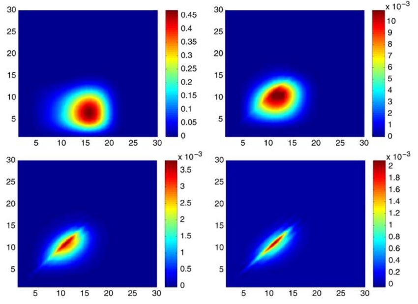
Figure 3 and 4 show the SPMCHF solution for this example. Neither SPHF nor SPMCHF
require initial estimates so the first calculation was for a Hartree Fock calculation for Mg
3s3d 1 D. The output was then used in the second multiconfiguration run as input to serve
as initial estimates and the first level varied only the 3p orbital, not present in the input.
Then the second varied all orbitals with excellent results as reported.
At this time, the SPMCHF program for multiconfiguration wave functions has not yet
been been fully tested. Through the use of the term=jj command-line option, the fully
relativistic DBSR - HF code can be used as an average energy level (EAL) approximation.Atoms 2021, 9, 50 11 of 14
Atoms 2021, 1, 0 11 of 14
MCHF WAVE FUNCTIONS FOR Mg Z = 12.0
Core = 1s( 2) 2s( 2) 2p( 6)
Other Orbitals = 3s~3d
Level 1: MCHF_parameters
----------------------
Step-size (h) 0.25000
Spline order (ks) 4
Size of basis (ns) 43
Maximum radius 256.79
SCF convergence tolerance 1.00D-11
Orbital convergence tolerance 1.00D-05
Orbital tail cut-off 1.00D-05
Orbitals varied all, all
SCF Phase
DeltaE =-0.17171D+02 Weighted total energy = -192.1383765929
DeltaE =-0.55311D+01 Weighted total energy = -197.6694874160
DeltaE =-0.89908D+00 Weighted total energy = -198.5685626677
DeltaE =-0.31594D+00 Weighted total energy = -198.8845019714
ALL_NR Phase
DeltaE = -0.4492D+00 Weighted total energy = -199.3336968207
DeltaE = -0.8426D-01 Weighted total energy = -199.4179608981
DeltaE = -0.8718D-02 Weighted total energy = -199.4266784165
DeltaE = -0.6904D-05 Weighted total energy = -199.4266853209
DeltaE = -0.7562D-07 Weighted total energy = -199.4266853965
DeltaE = -0.2549D-10 Weighted total energy = -199.4266853965
TOTAL ENERGY (a.u.) -199.426685396493866
Ratio -2.000000645930774
Level 2: MCHF_parameters
----------------------
Step-size (h) 0.12500
Spline order (ks) 8
Size of basis (ns) 78
Maximum radius 139.13
SCF convergence tolerance 1.00D-15
Orbital convergence tolerance 1.00D-08
Orbital tail cut-off 1.00D-08
Orbitals varied all, all
ALL_NR Phase
DeltaE = -0.3474D-04 Weighted total energy = -199.4267518942
DeltaE = 0.2993D-10 Weighted total energy = -199.4267518941
DeltaE = 0.6821D-12 Weighted total energy = -199.4267518941
TOTAL ENERGY (a.u.) -199.426751894120116
Ratio -1.999999999999927
Figure 3. Computer output of a Hartree–Fock calculation for the Mg [Ne] 3s3d 1 D wave function.
Figure 3. Computer output of a Hartree–Fock calculation for the Mg [Ne] 3s3d 1 D wave function.Atoms 2021, 9, 50 12 of 14
Atoms 2021, 1, 0 12 of 14
MCHF WAVE FUNCTIONS FOR Mg Z = 12.0
Core = 1s( 2) 2s( 2) 2p( 6)
Other Orbitals = 3s 3d~3p
Level 1: MCHF_parameters
----------------------
Step-size (h) 0.12500
Spline order (ks) 8
Size of basis (ns) 78
Maximum radius 139.13
SCF convergence tolerance 1.00D-15
Orbital convergence tolerance 1.00D-08
Orbital tail cut-off 1.00D-08
Orbitals varied =1, all
SCF Phase
DeltaE =-0.59389D-02 Weighted total energy = -199.4326908631
DeltaE =-0.15426D-02 Weighted total energy = -199.4342334760
DeltaE =-0.60072D-06 Weighted total energy = -199.4342340767
DeltaE =-0.38938D-11 Weighted total energy = -199.4342340767
ALL_NR Phase
DeltaE = -0.5324D-02 Weighted total energy = -199.4395583266
DeltaE = -0.8646D-03 Weighted total energy = -199.4404229110
DeltaE = -0.1338D-03 Weighted total energy = -199.4405567000
DeltaE = -0.1961D-04 Weighted total energy = -199.4405763067
DeltaE = -0.2794D-05 Weighted total energy = -199.4405791006
DeltaE = -0.3935D-06 Weighted total energy = -199.4405794941
DeltaE = -0.5516D-07 Weighted total energy = -199.4405795492
DeltaE = -0.7719D-08 Weighted total energy = -199.4405795569
DeltaE = -0.1079D-08 Weighted total energy = -199.4405795580
DeltaE = -0.1517D-09 Weighted total energy = -199.4405795582
DeltaE = -0.2049D-10 Weighted total energy = -199.4405795582
DeltaE = -0.3467D-11 Weighted total energy = -199.4405795582
DeltaE = 0.5400D-12 Weighted total energy = -199.4405795582
...
TOTAL ENERGY (a.u.) -199.440579558185400
Ratio -2.000000000000509
1 ) = c Φ (3s3d 1 D ) +
Computeroutput
Figure4.4.Computer
Figure outputfor
formulticonfiguration
multiconfiguration calculation for Ψ
calculation for Ψ((3s3d
3s3d 1D
D ) = c11 Φ(3s3d 1 D ) +
c2 Φ(3p 2 1 1
D ). Calculations are for Mg [Ne]3s3d 1 D using the radial functions from Figure 3 as
2 1
c2 Φ(3p D ). Calculations are for Mg [Ne]3s3d D using the radial functions from Figure 3 as
initial estimates.
initial estimates.
8.8. Concluding
ConcludingRemarksRemarks
The
Thespline
splinecodes
codesreviewed
reviewed in in this
this article
article were
were developed
developed in in the
the last
last 20
20 or or soso years.
years.
For
Forbound
boundstate
stateproblems,
problems,the theGRASP
GRASP code,code, for
for example [20],
[20], based
based on on finite
finite difference
difference
methods
methodsand andan anorthonormal
orthonormal orbital
orbital basis,
basis, is
is extensively used forfor complete
complete spectraspectrain- in-
cluding
cludingrelatively
relativelyhighly
highly excited
excited levels
levels [35]
[35] and
and certain heavy elements,
elements, primarily
primarily for for
highly
highlyionised
ionisedsystems
systemswherewherevalence
valence correlation
correlation can be dealt with
with and
and thethe effect
effectof ofcore
core
correlation
correlationon onspectra
spectraandandother
otherproperties
properties is is limited. with its
limited. SPMCHF with its greater
greater flexibility
flexibility
still
stillneeds
needstotobe betested
testedon onlanthanides
lanthanides and and actinides
actinides with two open
open shells
shells (n (n = = 4,4,55 for
for
lanthanides
lanthanidesand andnn==5,5,66for foractinides)
actinides) where
where natural
natural orbital transformation
transformation could couldproveprove
useful
usefulininconnection
connectionwith withorthonormal
orthonormal radial
radial functions
functions [36]. Multiple
Multiple ff-orbitals
-orbitals couldcouldalso
also
bebeaachallenge
challengefor forBSR inthat
BSRin thatthethenumber
number of of determinants
determinants can increase
increase rapidly.
rapidly.
InIn1984,
1984,itittook
took254254seconds
secondsto toexecute
execute aa numerical
numerical HF program for for Ra
Ra 7s 7s22 11SSononaaVAX
VAX
11/780;inin1987,
11/780; 1987,22seconds
secondson onaaCray
Cray X-MP;
X-MP; and
and in 1993, 1 s on a Dec
Dec Alpha,
Alpha, which whichwas was
a apopular
popularcomputer
computeratatits itstime.
time. Thus
Thus time
time (cost)
(cost) is no longer an important
important factor
factor butbutrather
rather
easeofofuse
ease useand
andreliability.
reliability.TheThesame
same isis not
not true
true when accurate wavewave functions
functions are areneeded
neededAtoms 2021, 9, 50 13 of 14
for many-electron systems for different atomic properties. Important now is how well an
algorithm can be made parallel, and how efficiently memory usage can be managed.
The present paper has been about non-relativistic calculations. Relativistic methods
are similar, except that the decision to represent large and small components of radial
functions by splines of different order, automatically implies that every Slater integral is the
sum of four integrals. This decision was important in BSR [2] in that it eliminated spurious
solutions in the R-matrix and was also used for DBSR - HF. However, is it the most efficient
solution of the problem? For a grid of nv intervals, the number of independent basis
functions is nv + k s − 1. Thus, by going from k s to k s − 1, the number of independent basis
states decreases. The spurious solutions generally are higher in the spectrum. For bound
state solutions, the asymptotic conditions are such that both the large and small components
and their derivatives go to zero. In fact, in non-relativistic calculations, applying both
conditions stabilises the solution at large r. Further study might be appropriate.
Funding: This research was funded by Canada NSERC Discovery Grant 2017-03851.
Data Availability Statement: Not applicable.
Acknowledgments: Much of the spline research described here was performed over many years at
Vanderbilt University with funding support from the Division of Chemical Science, Geosciences,
and Bioscience, Office of Basic Energy Sciences, Office of Science, and the U.S. Department of Energy.
Some of the program development was performed while at the Atomic Physics Division, National
Institute of Standards and Technology, Gaithersburg, and Maryland 20899-8422. The author very
much appreciated Professor Michel R. Godefroid’s comments and suggestions for this paper.
Conflicts of Interest: The author declares no conflict of interest.
References
1. Zatsarinny, O. A general program for computing matrix elements for atomic structure with nonorthogonal orbitals. Comp. Phys.
Commun. 1996, 98, 235–254. [CrossRef]
2. Zatsarinny, O. BSR: B-spline atomic R-matrix codes. Comput. Phys. Commun. 2006, 174, 273–356. [CrossRef]
3. Froese Fischer, C. A B-spline Hartree-Fock program. Comput. Phys. Commun. 2011, 182, 1315–1326.
4. Igarashi, A. B-Spline Expansions in Radial Dirac Equation. J. Phys. Soc. Jpn. 2006, 75, 114301. [CrossRef]
5. Igarashi, A. Kinetically balanced B-spline expansions in radial Dirac equation. J. Phys. Soc. Jpn. 2007, 76, 05431. [CrossRef]
6. Froese Fischer, C.; Zatsarinny, O. A B-spline Galerkin method for the Dirac equation. Comput. Phys. Commun. 2009, 180, 879–886.
[CrossRef]
7. Zatsarinny, O.; Froese Fischer, C. DBSR—A B-spline Dirac-Hartree-Fock program. Comput. Phys. Commun. 2016, 202, 287–303.
[CrossRef]
8. Hartree, D.R. The Calculations of Atomic Structures; Springer: New York, NY, USA, 1957.
9. Roothaan, C.C.J. New Developments in Molecular Orbital Theory. Rev. Mod. Phys. 1951, 23, 69–89. [CrossRef]
10. Bachau, H.; Cormier, E.; Decleva, P.; Hansen, J.E.; Martin, F. Applications of B-splines in atomic and molecular physics. Rep. Prog.
Phys. 2001, 64, 1815–1942. [CrossRef]
11. de Boor, C. A Practice Guide to Splines; Springer: New York, NY, USA, 1985.
12. Johnson, W.R.; Sapirstein, J. Computation of Second-Order Many-Body Corrections in Relativistic Atomic Systems. Phys. Rev.
Lett. 1986, 57, 1126. [CrossRef]
13. Froese Fischer, C. A general multiconfiguration Hartree-Fock program. Comput. Phys. Commun. 1978, 14, 145–153. [CrossRef]
14. Froese Fischer, C.; Tachiev, G.; Gaigalas, G.; Godefroid, M.R. An MCHF atomic-structure package for large-scale calculations.
Comput. Phys. Commun. 2007, 176, 559–579. [CrossRef]
15. Hibbert, A.; Froese Fischer, C.; Godefroid, M.R. Non-orthogonal orbitals in MCHF or configuration interaction wave functions.
Comput. Phys. Commun. 1988, 51, 282–293. [CrossRef]
16. Froese Fischer, C.; Parpia, F.A. Accurate spline solutions of the radial Dirac equation. Phys. Lett. A 1993, 179, 198–204. [CrossRef]
17. Qiu, Y.; Froese Fischer, C. Integration by cell algorithm for Slater integrals in a spline basis. J. Comput. Phys. 1999, 156, 257–271.
[CrossRef]
18. Froese Fischer, C. Concurrent vector algorithms for spline solutions of the helium pair equation. Int. J. High Perform. Comput.
Appl. 1991, 5, 5–20. [CrossRef]
19. Froese Fischer, C. B-splines in variational atomic structur calculations. Adv. At. Mol. Phys. 2007, 55, 539–550.
20. Froese Fischer, C.; Gaigalas, G.; Jönsson, P.; Bieroń, J. GRASP2018—A Fortran 95 version of the General Relativistic Atomic
Structure Package. Comput. Phys. Commun. 2019, 237, 184–187. [CrossRef]
21. LAPACK Library. Available online: http://www.netlib.org/lapack/ (accessed on 28 July 2021).Atoms 2021, 9, 50 14 of 14
22. LINPACK Library. Available online: http://www.netlib.org/linpack/ (accessed on 28 July 2021).
23. Froese Fischer, C.; Idrees, M. Spline algorithms for continuum functions. Comput. Phys. 1989, 3, 53–58. [CrossRef]
24. Froese Fischer, C.; Idrees, M. Spline methods for resonances in photoionisation cross sections. J. Phys. B At. Mol. Opt. Phys. 1990,
23, 679. [CrossRef]
25. Brage, T.; Froese Fischer, C.; Miecznik, G. Non-variational, spline-Galerkin calculations of resonance positions and widths, and
photodetachment and photoionization cross sections for H− and He. J. Phys. B At. Mol. Opt. Phys. 1992, 25, 5289–5314. [CrossRef]
26. Brage, T.; Froese Fischer, C. Spline-Galerkin methods for Rydberg series, including Breit-Pauli effects. J. Phys. B At. Mol. Opt.
Phys. 1994, 27, 5467–5484. [CrossRef]
27. Xi, J.; Froese Fischer, C. Cross section and angular distribution for the photodetachment of He− 1s2s2p 4 Po below the He n = 4
threshold. Phys. Rev. A 1996, 53, 3169–3177. [CrossRef]
28. Xi, J.; Froese Fischer, C. Photodetachment cross-section of He- (1s2s2p 4 Po ) in the region of the 1s detachment threshold. Phys.
Rev. A 1999, 59, 307–314. [CrossRef]
29. Xi, J.; Froese Fischer, C. Cross section and angular distribution for photodetachment of Be- 1s2 2s2p2 4 P. J. Phys. B At. Mol. Opt.
Phys. 1999, 32, 387–396. [CrossRef]
30. Zatsarinny, O.; Froese Fischer, C. The use of basis splines and non-orthogonal orbitals in R-matrix calculations: Application to Li
photoionization. J. Phys. B At. Mol. Opt. Phys. 2000, 33, 313–341. [CrossRef]
31. Froese Fischer, C.; Guo, W. Spline algorithms for the Hartree-Fock equation for the helium ground state. J. Comput. Phys. 1990, 90,
486–496. [CrossRef]
32. Froese Fischer, C.; Guo, W.; Shen, Z. Spline methods for multiconfiguration Hartree-Fock calculations. Int. J. Quantum Chem. 1992,
42, 849–867. [CrossRef]
33. SPMCHF. Available online: http://github.com/compas/spmchf(accessed on 28 July 2021).
34. Zatsarinny, O.; Drake Umiversity. Private communication, 1 May 2016.
35. Li, W.; Amarsi, A.M.; Papoulia, A.; Ekman, J.; Jönsson, P. Extended theoretical transition data in C I – IV. Mon. Not. R. Astron. Soc.
2021, 502, 3780–3799. [CrossRef]
36. Schiffmann, S.; Godefroid, M.; Ekman, J.; Jönsson, P.; Froese Fischer, C. Natural orbitals in multiconfiguration calculations of
hyperfine-structure parameters. Phys. Rev. A 2020, 101, 062510. [CrossRef]You can also read