Transportation Networks and the Rise of the Knowledge Economy in 19th Century France - Economic History Society

Transportation Networks and the Rise of the Knowledge
 Economy in 19th Century France∗

 Georgios Tsiachtsiras†
 Latest version here

 February 16, 2022
 Abstract

 This paper exploits an episode of French history to study the relationship between the roll-out of rail-
 roads and the rise of the knowledge economy. I take advantage of the exogenous variation in railway
 access arising from a straight line time variant instrument, to document that access to rail network
 increases the innovation activity at the canton level. I explore access to knowledge as an underlying
 mechanism behind the main results. I find that the innovation performance of a given canton depends
 crucially on how well connected is through the rail and canal network to other cantons inhabited by
 inventors. Next, using text analysis techniques, I am able to determine the technology of each patent
 application in the historical database of the National Institute of Industrial Property of France and to
 explore the role of a global city, such as Paris, on the diffusion of new technologies. Finally, I introduce
 a back of the envelope exercise based on canals to show that in the absence of railroads the invention
 rate of the French cantons would have been, on average, 21.3% lower.

 Keywords: innovation, patent data, railroads, access to knowledge
 JEL classification: L92, N73, O31, O33, P25, R12

 ∗ I would like to thank from the bottom of my heart, Rosina Moreno and Ernest Miguelez for their guidance and support at all the stages
of this paper. Special thanks to Anastasia Litina and Sergio Petralia for helpful discussions and comments. I am grateful to Steeve Gallizia,
Christophe Mimeur, Teresa Sanchís and Nicolas Verdier for sharing with me their historical datasets. I would like to express my gratitude to
Richard Hornbeck for sharing with me his replication files. I have benefited from the comments of Thomas Piketty, Sascha O. Becker, Mara
Squicciarini, Erik Hornung, Yanos Zylberberg, Diogo Britto, Carlo Schwarz, Jan Bakker, Carlos Serrano, Francesco Quatraro, Stefano Breschi,
Denis Cogneau, Laurent Bonnaud, Tommaso Ciarli, Cédric Chambru, Zelda Brutti, Mario Holzner, Markus Lamp, Marina Chuchko, Miquel-
Ángel Garcia-Lopez, Ester Manna, Xavier Fageda, Emilie Bonhoure, Abel Lucena, Mercedes Teruel, Dolores Añon Higon, András Jagadits,
Vera Rocha, Alexander Klein, Fabian Gaessler, Ivan Yotzov, Nikos Benos, Nikos Tsakiris, Nikolaos Mylonidis, Paraskevi Salamaliki, Stella Tsani,
Dirk Martignoni, Bjoern Brey, Giuseppe Cappellari, Filippo Tassinari, Eric Melander, Michel Philippe Lioussis, Ivan Hajdukovic, Emanuele
Caggiano, Maria Teresa Gonzalez, Emanuele Cagnolo, Shreekanth Mahendiran, Anthi Kiouka, Christopher Esposito, Carolin Ioramashvili,
Diego Cagigas and the participants of the 10th PhD-Student Workshop on Industrial and Public Economics (2022), the SEG Winter Workshop
in the Geography of Innovation (2022), the Economic History Seminar at Paris School of Economics (2021), the F4T Seminar Series (Bocconi
University, 2021), the Young Economist Symposium 2021 (sponsored by Columbia, NYU, UPenn, Princeton and Yale), the European Winter
Meeting of the ES (2021), the IP and Innovation Virtual Seminar (2021), the AYEW Infrastructure Workshop (organized by the Monash Univer-
sity and the University of Warwick, 2021), the 15th North American Meeting of the Urban Economics Association (Arizona University, 2021),
the HEC Paris Entrepreneurship Workshop (2021), the WU Economic & Social History Research Seminar (2021), the 6th Summer School on
Data & Algorithms for ST&I studies (organized by the Aristotle University and the KU Leuven, 2021), the DRUID 2021 (Copenhagen Business
School), the PhD - Economics Virtual Seminar, the 11th ifo Dresden Workshop on Regional Economics (2021), the EPIP Conference (2021),
the XXIII Applied Economics Meeting (Universitat de València, 2021), the Symposium of the Spanish Economic Association (2021), Virtual
Meeting of the Urban Economics Association (2020), the 13th RGS Doctoral Conference in Economics on Regional Disparities and Economic
Policy in Europe (Technische Universität of Dortmund, 2020), the 5th Geography of Innovation Conference (University of Stavanger, 2020), the
7th International PhD Workshop in Economics of Innovation, Complexity and Knowledge (University of Turin, 2020), the Webinar Series of
University of Ioannina, and the 4th Summer School in Economics (University of Ioannina, 2019). Financial support from Agaur (FI-DGR). Any
remaining errors are mine.
 † Tsiachtsiras: Ph.D. candidate, University of Barcelona School of Economics; Department of Statistics, Econometrics, and Applied Eco-
nomics, Barcelona 08034, Spain. email: gtsiachtsiras@ub.edu

 1

"There is no country in the world where so small a proportion of the capital invested within
 the last forty years in canals and railroads, has been wasted or where traveling is safer,
 or in which travel and trade are accommodated at more reasonable rates than in France"
 (Moncure Robinson, American Philosophical Society, 1880)

1 Introduction
Productivity growth depends on two elements: new ideas bringing new technologies, and the diffusion
of these ideas among people and places. The rate of a person’s learning at any task depends on the envi-
ronment in which the person is exposed (Lucas, 1988; Lucas and Moll, 2014; Bell et al., 2019). As a result
high skilled people tend to co-locate in order to benefit from a faster rate of contact with other individu-
als at the same level of skills (Marshall, 1890; Glaeser, 1999; Moretti, 2021). This process is driven by the
costly nature of generating new ideas (Bloom et al., 2020) which may be translated to new inventions.
However, transport infrastructure investments across cities may provide a broader reach to otherwise
localized knowledge spillovers (Jaffe et al., 1993; Murata et al., 2014) by lowering the cost of exchanging
ideas among places (Agrawal et al., 2017; Dong et al., 2020).
 Connecting places via transportation networks is essential in order to promote knowledge diffusion
across the space, and hence long-term economic growth. Over the last few decades, the World Bank
has spent a large proportion of money on funding infrastructure investments (World Bank, 2007, 2013,
2017).1 Despite an emphasis on reducing transportation costs, we lack empirical evidence on understand-
ing how transportation infrastructure projects can actually create meaningful connections to places that
matter in terms of boosting innovation performance and strengthening channels related to the diffusion
of knowledge.
 In this paper, I exploit an episode of French history to study the impact of the largest-scale construction
of French railroads on innovation performance. Over the second half of the 19th century, railroad con-
struction transformed the French economy. Railways generated economic relations and cultural environ-
ments, stimulated commerce and created new economic opportunities. The creation of the rail network
changed the perception of time (Schwartz et al., 2011). According to Thévenin et al. (2013) a striking
example of this transformation is the travel time between Paris and Marseille. In 1814, the duration of
this trip was four to five days while in 1857, this trip needed about 13 hours.
 Remarkably, the roll-out of the network coincided with a rise of innovation activity. Up to 1850, the
number of patent applications owned by inventors in the historical French patent database was 22,978.
From 1850 to 1902, this figure increases to 285,597. Some of the greatest inventions in history took place
in France during the second half of the 19th Century, such as Louis Pasteur’s inventions for wine and beer
pasteurization in 1865 and 1871, respectively. Another example is the invention of the French chemist,
Charles Frederic Gerhardt who, in 1853, was the first person to prepare acetylsalicylic acid (aspirin).
Lastly, the very first patented film camera was invented by Louis Le Prince in 1888.
 I use rich historical data to construct a panel dataset at the canton level for France (2,925 cantons) over
the period 1850-1890.2 I combine a very recent dataset of communes with access to rail station in the 19th

 1 Based on reports of 2007, 2013 and 2017, the World Bank spent approximately $105 billion on transport-related projects.
 2I include only the cantons from the mainland of France.

 2

century (Mimeur et al., 2018) with the historical patent applications database of the National Institute
of Industrial Property office (hereinafter, the INPI) (INPI, 2019) for the period 1850-1890 to construct a
unique dataset.3 The historical patent database of INPI is still fairly unexplored. Previous papers have
used the INPI database during the first half of 19th century to study the effect of technology transfer from
Britain to France (Nuvolari et al., 2020), the influence of the patent system on economic performance
(Galvez-Behar, 2019), the role of women in enterprise and invention in France (Khan, 2016) and the
impact of labor scarcity on technology adoption and innovation (Raphael, 2022).
 Equipped with this dataset, this paper focuses on the expansion of the French railroad network which
provides a unique setting to identify the causal impact of transport infrastructure on innovation out-
comes. I use the three different French railway plans over the course of the 19th century to construct a
time variant straight line instrument. I document that access to a rail station increases a canton’s inno-
vation activity. For robustness analysis, and to complement the instrumental variance approach, I apply
an inconsequential units approach based on the randomly chosen subset of municipalities that received
railway access because they lie on the most direct route between the nodal destinations used to create
the straight line instrument. In addition, I exploit the richness of the patent data to create a falsification
exercise in which I regress the distance to rail stations on invention rate of the cantons over the period
1800-1840 one decade prior to the actual arrival of railroads. I do not report a significant effect meaning
that future railroads are not associated with past innovation activity, at least the decades immediately
prior to the sample period. I interpret this as evidence that my results are not driven by pre-trends re-
lated to the railroads and innovation performance. Moreover, in the Appendix A, I provide a conventional
difference-in-differences regression model with staggered treatment using a binary indicator as an inde-
pendent variable, switching to 1 if the canton has access to a rail station. This design covers the period
1800-1890 allowing me to control for a long period of time, 1800-1840, before the arrival of railroads,
when none of the cantons have access to a rail station. Finally, in the Appendix A, I explore cross section
variation for every decade over the period 1850-1890 to identify the year that railroads started to have an
impact on the patenting rate and to test the validity of the instrument by decade.
 In a second step, I explore the mechanism behind the main results. This paper adds to the literature by
using the rationality of the "market access" framework, developed by Donaldson and Hornbeck (2016),
to provide a supply side mechanism related to potential interactions (Akcigit et al., 2018) and knowledge
spillovers (Jaffe et al., 1993) among the inventors residing in different cantons. Rather than using popu-
lation in the market access index, the paper uses the number of inventors. The potential interactions and
spillovers among inventors residing in different cantons could occur by establishing less costly routes,
due to infrastructure improvements, within mainland France. I call this mechanism access to knowl-
edge. A previous attempt in the literature uses a market access framework (Perlman, 2015) to identify
the mechanism that boosts innovation performance. Other papers in the literature (Agrawal et al., 2017;
Andersson et al., 2021; Inoue and Nakajima, 2017; Wong, 2019; Gao and Zheng, 2020; Dong et al., 2020;
Sun et al., 2021; Hanley et al., 2021; Komikado et al., 2021; Cui et al., 2020; Huang and Wang, 2020) pro-
vide evidence on how transportation networks facilitate the diffusion of knowledge but without directly
connecting the knowledge diffusion mechanism to innovation performance. Prior literature explores also
supply side mechanisms on innovation performance like past co-inventors, inventors in the same firm,

 3 The patent database is available on request.

 3

inventors in the same geographical region (Akcigit et al., 2018), degree and closeness centrality of a city
(Yao et al., 2020), collaborations (Inoue and Liu, 2015; MingJi and Ping, 2014; Guan et al., 2005) and mo-
bility of the inventors (Rahko, 2017). To the best of my knowledge, this is the first attempt to establish a
supply side mechanism which connects via a transportation network a region’s innovation performance
to the outside world.
 Finally, this paper uses the unique setting of France to introduce as a special case the importance for the
inventors of a given canton to have a less costly connection to a global city such as Paris. Prior literature
argues that Paris can work as a gatekeeper of knowledge that connects the national innovation system to
global innovation networks (Miguelez et al., 2019). This is confirmed by the fact that inventions in Paris
are more diverse and spread across the different technologies (Kogler et al., 2018). Paris was considered
to be an important node in the global economic system also in the 19th century. Five World Fairs took
place in Paris during the second half of 19th century. The literature has explored the crucial effect of
World Fairs on technological change (Moser, 2005). A lot of inventors from around the world presented
their inventions at the World Fairs. Paris acted like a link for the cities of France to the outside world.
However, for only a small sample of patent applications, INPI database contains information about their
technological class. In order to explore this special case, I assign technological classes to the remaining
patent applications in the historical database of INPI. I assemble a vocabulary which is based on key
words from the titles of the patent applications for which I have their technological class. Using this
vocabulary, I can assign technological classes to all the patent applications in the INPI database.
 This paper directly speaks to the literature about transportation networks and innovation activity. Stud-
ies that are close to my research include the papers by Perlman (2015), Agrawal et al. (2017) and An-
dersson et al. (2021). Perlman (2015) establishes a relationship between network access and innovative
activity in the USA over the 19th century. Agrawal et al. (2017) find that the stock of highways has a
positive effect on patenting in metropolitan statistical areas of the USA. Finally, Andersson et al. (2021)
explore the effect of the Swedish railroad on patent activity over the period 1830-1910. They assert that
network access fosters innovation activity. They find solid evidence that independent inventors start to
specialize in specific technologies when they enter the market. General railroad access helps the inventors
to develop ideas beyond the local economy and invent in new technological classes.
 There is a growing body of literature exploring the interplay between infrastructure and economic
outcomes from a historical perspective. Railroads in the USA, Sweden, England, Wales and Switzerland
transformed all towns into new places. They managed to lure banks and to increase urbanization (Atack
et al., 2008, 2009; Atack and Margo, 2009; Berger and Enflo, 2017; Büchel and Kyburz, 2020; Bogart et al.,
2022) and are responsible for the growth and the economic development of US and Nigeria cities (Nagy,
2016; Okoye et al., 2019). Railroads also have a significant impact on the development of the agricul-
tural sector (Donaldson and Hornbeck, 2016; Donaldson, 2018) and on fertility and human capital (Katz,
2018). Transportation linkages have an adverse effect on health in the rural US (Zimran, 2019). Railroads
manage to boost manufacturing productivity in US (Hornbeck and Rotemberg, 2019; Pontarollo and Ric-
ciuti, 2020). Finally, the steam railway led to the first large-scale separation of workplace and residence
(Heblich et al., 2020).
 In general, infrastructure networks can affect the economy through different channels. The realloca-
tion of road investments after the division of Germany created regional income inequalities in terms of

 4

GDP per capita (Santamaria, 2020). Highways affect population and employment (Baum-Snow, 2007;
Duranton and Turner, 2012). Lastly, the adoption of the steamship between 1850 and 1900 boosted the
globalization of trade (Pascali, 2017).
 In addition, this paper proposes that targeted investments to infrastructure projects can facilitate access
to big cities. This direct policy may level out the persistent inequalities between urban and rural areas. It
may increase the probability of smaller cities to innovate in new patent classes. Recent papers rise con-
cerns about the correct allocation of infrastructure funds (Flyvbjerg, 2009) and the proper circumstances
for such projects to be efficient (Crescenzi et al., 2016).
 Lastly, given the setting of the analysis, this paper adds to the literature on the economic progress
and economic history of France around the turn of the 19th and 20th century by studying the impact of
railroads on technological progress. Other papers in the literature explore as determinants of economic
growth religiosity (Squicciarini, 2020; Lecce et al., 2021), knowledge elites (Squicciarini and Voigtländer,
2015), trade (Juhász, 2018), adoption of technological breakthroughs (Juhász et al., 2020), large income
shock of the phylloxera (Banerjee et al., 2010), emigration intensity (Franck and Michalopoulos, 2017),
population shifts (Talandier et al., 2016), early industrialization through the adoption and persistence of
unskilled-labor-intensive technologies (Franck and Galor, 2019) and fertility rates Daudin et al. (2019).
One previous attempt related to railroads focuses on the effect of railroads on population distribution in
France, Spain, and Portugal from 1870 to 2000 (Mojica and Martí-Henneberg, 2011).
 The rest of the paper is organized as follows: Section 2 contains the historical background, section 3
presents the data, section 4 shows the empirical strategy, section 5 presents the main results, section 6
explores the mechanism and section 7 concludes.

2 Historical Background
2.1 Railroads
The first railway line in France was built in 1828 by mining companies to connect St. Etienne to the Loire
River. They used this line to transfer coal. The first line for passengers was opened in 1837. It was a short
line from Paris to Le Pecq (Dunham, 1941). At the time, France was already lagging behind Britain and
Belgium. In 1842 Britain had 1,900 miles of railways in operation while France had only 300 (Lefranc,
1930).
 After the success of the first line, the French government saw the importance of a national railway net-
work. However, the next attempt for constructing a rail line between Paris and Versailles was unsuccess-
ful. Two different companies each built a line to connect Paris with Versailles but they failed financially.
The government recognized the problem of rivalry between local interests (Dunham, 1941). Although
the government was aware of the importance of a national railroad, it did not provide funding until 1842
(Ratcliffe, 1976).
 According to Dunham (1941) the planning of rail network was given to Corps des ponts et chaussees, an
organization of highly trained engineers which was in charge for major infrastructure projects in France.
The expansion of railroads during the period 1840-1860 was based on Legrand Star, a design by the Corps
des ponts et chaussees. According to Legrand plan, the purpose of the government was to connect major
communes, borders, and coastlines with Paris. In 1865, based on the Migneret law, the government estab-

 5

lished direct lines connecting all the prefectures. The final expansion of the rail network was constructed
according to the Freycinet plan which was introduced in 1878 (Thévenin et al., 2013).
 The most important railroad expansion occurred between 1860 and 1900 when 45,000 km of rail lines
were built. The final phase ran until the 1930s and by the end of this phase 56,000 km of railroad were in
operation (Thévenin et al., 2013). The introduction of motor vehicles at the end of the 1930s limited the
expansion of the railroad network.

2.2 Patent System
Great Britain, France and the United States were the first countries to adopt legislation on patents in 1791
(Macleod, 1991; Galvez-Behar, 2019). In France, prior to the establishment of a patent legislation, and
more specifically during the 18th century, patent applications were known as "les privileges" and were
granted by the king and registered by the parliament in Paris (Macleod, 1991). In addition, inventors
received remarkable awards for their inventions, such as national or local production, a lifelong pension or
tax exemption. Lastly, a major difference between the English and French system was that the application
procedure was far more severe in the latter case (Macleod, 1991).
 In 1791, Boufflers’ bill became the first Patent Act in France establishing three different categories for
patenting: 1) Patents for invention, 2) Patents for improvement and 3) Patents for importation. The
patents were granted from five until fifteen years. The name of the inventions changed to "brevets de
invention". However, their cost was prohibitive. Apart from the initial cost, several taxes were added
over the course of the examination process. The patent system did not facilitate the spread of patenting,
because a lot of inventors could not afford the high cost (Galvez-Behar, 2019).
 The rise of patenting activity was underpinned by the introduction of a patent law in 1844. This leg-
islation allowed the inventors to export their patents to foreign countries and also changed the method
of payment for inventors enabling patentees to spread the payment of the tax over the entire duration of
their patent (Galvez-Behar, 2019).

3 Data
3.1 Railroad Data
The data on communes with a rail station over the period 1860-1920 come from Mimeur et al. (2018). It
is a very detailed database that contains five variables of interest for all the communes.4
 I make use of an historical image with rail lines until 1860 to add one additional decade to my sample.5
I extract the lines from the image that were already established until 1850 to identify the communes that
had a rail station in 1850. In order to do that, I rely on the historical rail station data of 1860 from Mimeur
et al. (2018) and I preserve only the communes which are crossed by a rail line of 1850. This exercise
allows me to identify the communes with a rail station in 1850.
Distance to Rail Station: It is the distance in km from any canton city point to the closest commune
centroid with access to a rail station.
 4 It contains a dummy variable of access (=1 if the commune has a rail station), a variable of the type of line, and three
variables with travel time to reach from any commune to Paris, regional centers and departmental centers.
 5 For more details see Figure D1 in the Appendix D.

 6

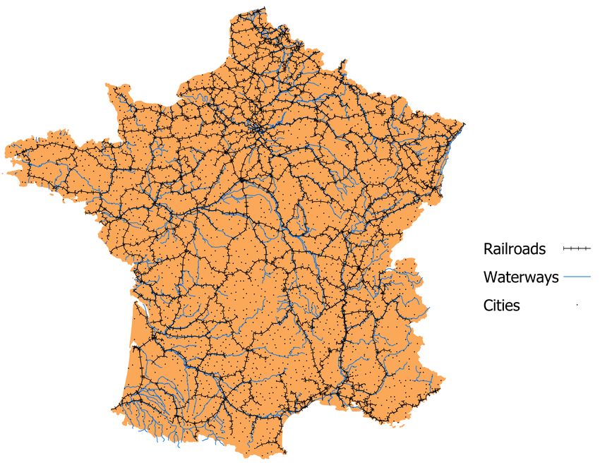
Furthermore, I attempt to create the historical rail line network of France. In the absence of high reso-
lution historical maps, I use the communes with rail stations in the period 1850-1890 and modern French
rail lines.6 Baum-Snow et al. (2017, 2018) argue that historical infrastructure networks are good predictors
and facilitate the construction of a lower cost and more modern infrastructure network. In this paper, I
use a modern infrastructure network to re-create an old one. I use a shapefile with the rail lines in the
period 2000-2020 (Jeansoulin, 2019) and a shapefile with the lines until 1992 (DIVA-GIS, 2020). Figure
1 shows the results of this exercise. According to the findings a significant development of rail network
occurred in France over the 19th century.

3.2 Canal Data and Ports
Aside from the railroads, France also developed a canal network. I make use of two sources of data to
identify the canal network of France.
 The first source of data on navigable waterways comes from Ryavec and Henderson (2017). It is a
shapefile developed by Jordi Marti Henneberg.7 This shapefile includes the canal network of France in
1850. The second source of data is the collection of historical maps of Chicago (2020) which contains very
detailed maps of the navigable waterways of France over the second half of 19th century.8 I digitized these
historical maps in QGIS. Figure 1 shows the expansion of canals. Next, I construct the indicator of access
to the canal network.
Access to Navigable Waterways: It is a binary indicator which switches to 1 for a canton if there is a canal
within 3 km distance from the city centroid. In the Appendix A, I apply robustness check with different
thresholds.
 In addition, I make use of a historical map from Rumsey (2020) collection, in order to identify the
ports of France in 1877.9 I complement this data with active ports over the period 1662-1855 from García-
Herrera et al. (2006). Their database focuses on the reconstruction of oceanic wind field patterns for
this period that precedes the time in which anthropogenic influences on climate became evident. They
include the variables "voyagefrom" and "voyageto" which contain the names of the places where the ship
departed from or sailed to. I apply geocoding on Stata (Zeigermann, 2018) and I identify 13 active ports
for France.10 I use the ports to construct the instrument for the IV approach.

3.3 Setting
I make use of the recent constructed shapefiles of Gay (2020), for the period 1870-1940. Over the sample
period, France did not experience any large changes in the national administrative system except for the
departments that became part of Germany. I base my analysis on the shapefile of 1870 which contains
2,925 cantons for mainland France.
 Next, I can determine the majority of the city areas in order to use the centroids of the cities. The first
data source is Perret et al. (2015), which contains the polygons of the cities, towns, domains and forts

 6 For
 more details see Figure D2 and Figure D3 in the Appendix D.
 7 Source:
 http://europa.udl.cat/projects/inland-waterways/
 8 For an example of the maps see Figure D4 in the Appendix D.
 9 For more details see Figure D4, Appendix D.
 10 At least one ship departed or sailed to these ports.

 7

Figure 1: Expansion of Railroads and Navigable Waterways

 (a) 1850 (b) 1860

 (c) 1870 (d) 1880 (e) 1890

 Notes: This figure shows the expansion of navigable waterways in France over the period 1850-
 1890. Source: the shapefile of canal network for 1850 comes from Ryavec and Henderson (2017)
 and for the period 1860-1890, it is based on author’s digitization of the historical maps from the
 Chicago (2020). The railroads lines are constructed by the author based on historical rail stations
 by Mimeur et al. (2018) and recent shapefiles of rail lines from DIVA-GIS (2020) and Jeansoulin
 (2019).

during the 18th century. For a given canton , I first use the cities within the polygon followed by the
towns, domains and forts. If a canton has more than one city, I keep the centroid of the largest city (by
area) as a reference point. The same rule applies in the case of a town, domain or fort. I determine the
location of 1,961 cities, 69 towns, 112 domains and 3 forts which corresponds to 2145 cantons, or 73.33%
of the sample. I complement my analysis using population raster file of 1840 from HYDE (2020). I use
the year 1840 because it is the closest available year before the arrival of railroads. Based on the second
source of data, I use QGIS to convert the raster file into pixels and for the remaining cantons, without a
reference point, I choose the pixel with the highest population value. Furthermore, I assign a reference
point in 738 cantons, which corresponds to 25.23% of the sample. For the remaining 42 cantons without
a reference point (1.44% of the sample), I use the centroid of the polygon. Figure 2 illustrates an example
of the empirical setting. The grey areas are the cantons and the red polygons are the city borders. The
black dots, within the red polygons, are the city centroids. The green dots are the rail stations, while the
blue lines are the navigable waterways. I believe that the use of these points, instead of the centroids of
the polygons, makes the analysis more realistic as they represent with a higher precision the location of
the cities.

3.4 Patent Data
The historical database of the INPI contains all the patent applications (409,324 applications with their
additions) covering the period 1791-1902. The database includes the application number of the patents,

 8

Figure 2: Setting

 Notes: This figure illustrates an example of the research setting of the paper.

the filing year, the name of the applicant(s), the commune, the street and number of the applicant(s),
the title of the patents and the expiry date of the patent applications. Additional details are included in
the database such as whether an application is a patent that was imported from abroad, the number of
additions of every patent application and the profession of the applicant.
 I restrict my sample only to applications with at least one inventor residing in France. I remove applica-
tions that belong only to firms using key words.11 Next, I exclude 116 applications without a filing date.
When one application has several improvements (additions), I do not consider the improvements, but
only the initial design. Finally, I exclude from the sample the patent applications that are importations
since it is more likely that the inventor was resident of another country and only the patent agent was in
France. I end up with 308,926 patent applications over the entire period. Figure 3 presents the evolution
of patent applications per capita over the sample period of the paper as well as the time trend for the
average distance to rail stations.
 With this information, I construct the following variables.
Number of patent applications: I calculate the total sum of patents for each decade from 1850 to 1890
like in Andersson et al. (2021).
Number of patent applications that received an addition: INPI database contains the number of ad-
ditions of each patent application. The patent law of 1844 gave the applicants the option to apply for
certificates of addition (Galvez-Behar, 2019) which allowed applicants to protect a minor improvement

 11 I exclude all the applications that have the words “COMPAN” or “COMPAGNI” or “SOCIETA” or “SOCIET” or
"GESELLSCHAFT" or "SYNDICAT" or "GESELLSCHAF" or "MANUFACTUR" in the applicant’s name.

 9

Figure 3: Innovation per Capita and Average Distance to Rail Stations

 Patents per Capita and Average Distance to Stations

 .002
 1 .8

 .0015
 Distance to Rail Stations

 Patents per Capita
 .6

 .001
 .4

 .0005
 .2 0

 0
 1850 1860 1870 1880 1890
 Year

 Distance to Rail Stations Patents per Capita

 Notes: Summary graph showing the time trend of patent applications per capita and average
 distance to rail station. Source: author’s computations based on the patent applications from INPI
 (2019) database, population from HYDE (2020) and rail stations from Mimeur et al. (2018).

to the initial patent throughout its term. An addition to the initial design costs an extra of 24 francs (Nu-
volari et al., 2020). As a quality measure of innovation, I restrict the sample of patents to the ones that
received an addition.
 Apart from the main database, INPI includes a sample of 38,527 patent applications with their tech-
nological field. These patents are divided in 20 main classes.12 For only this sample of patents, I have
information on their main class and their title. I use the "lsemantica" command in Stata (Schwarz, 2019)
to extract key words from the titles of the patent applications and then complement these key words with
additional words from the names of the main and sub classes of patent applications. Afterwards, I keep
the unique words among classes to create a vocabulary. Based on this vocabulary, I manage to assign
classes to the rest of the patent applications in the INPI database. More technical details regarding this
method and the vocabulary can be found in the Appendix C. Figure 4 illustrates the time trend for every
class. As a result of this analysis, I construct two more indicators of innovation.
Number of Novel Classes: It is the number of new technology fields in which a canton has at least one
invention in a given year
Stock of Classes: It is for every time period the number of technological classes that a canton already has
at least one invention.

 12 The 20 classes are: Agriculture, Alimentation Railways and Trams, Arts textile, Fibers and Yarns, Machines, Marine and
Navigation Construction, Public and Private, Mines and Metallurgy, Domestic Economy, Weapons, Road Transport, Instruments
of Precision and Electricity, Ceramics, Chemics, Lighting Heating Refrigeration and Ventilation, Clothes, Arts, Office Supplies
and Education, Medicine and Health, Articles and Various Industries.

 10

Figure 4: Applications by classes

 1500

 500 1000 1500 2000

 Arts textile, Fibers and Yarns
 600

 1000 2000 3000 4000
 0 200 400 600 800 1000
 Railways and Trams
 1000

 Alimentation
 400
 Agriculture

 Machines
 500

 200
 0

 0

 0

 0
 1820 1840 1860 1880 1900 1820 1840 1860 1880 1900 1820 1840 1860 1880 1900 1820 1840 1860 1880 1900 1820 1840 1860 1880 1900
 Year Year Year Year Year

 Construction, Public and Private
 500 1000 1500 2000
 100 200 300 400

 200 400 600 800

 800
 600
 Marine and Navigation

 Mines and Metallurgy

 Domestic Economy

 Road Transport
 200 400 600
 200 400
 0

 0

 0

 0

 0
 1820 1840 1860 1880 1900 1820 1840 1860 1880 1900 1820 1840 1860 1880 1900 1820 1840 1860 1880 1900 1820 1840 1860 1880 1900

 Articles and Various Industries Lighting, Heating, Refrigeration and Ventilation
 Year Year Year Year Year

 Instruments of Precision and Electricity

 3000

 1500
 1500
 800

 400
 200 400 600

 100 200 300

 2000

 1000
 1000
 Weapons

 Ceramics

 Chemics
 1000

 500
 500
 0

 0

 0

 0

 0
 1820 1840 1860 1880 1900 1820 1840 1860 1880 1900 1820 1840 1860 1880 1900 1820 1840 1860 1880 1900 1820 1840 1860 1880 1900
 Year Year Year Year Year
 Office Supplies and Education
 1000 1500 2000

 3000

 100 200 300 400

 100 200 300 400 500

 600
 Medicine and Health
 2000

 400
 Clothes

 Arts
 1000

 200
 500
 0

 0

 0

 0

 0
 1820 1840 1860 1880 1900 1820 1840 1860 1880 1900 1820 1840 1860 1880 1900 1820 1840 1860 1880 1900 1820 1840 1860 1880 1900
 Year Year Year Year Year

 Notes: Summary graph presenting the evolution of patent applications by classes. If an appli-
 cation has several classes, I allocate one application to all of them. The classes are: Agriculture,
 Alimentation Railways and Trams, Arts textile, Fibers and Yarns, Machines, Marine and Naviga-
 tion Construction, Public and Private, Mines and Metallurgy, Domestic Economy, Weapons, Road
 Transport, Instruments of Precision and Electricity, Ceramics, Chemics, Lighting Heating Refrig-
 eration and Ventilation, Clothes, Arts, Office Supplies and Education, Medicine and Health, Ar-
 ticles and Various Industries. Source: author’s computations based on patent applications from
 INPI (2019).

 Next, in order to be sure that I do not double count inventors residing in the same canton, I apply a
simple applicant disambiguation based on their name, surname and address. This exercise allows me
to assign a unique identifier to the inventors. I apply fuzzy matching (Raffo, 2020) on the name and
surname of applicants residing in the same street. I then consider the applicants with a matching score
over 73% to be the same person. I identify 334,504 unique applicants from 353,017 patent applications.
Even though the disambiguation is simple and "kills" the mobility of the inventors, since one of the criteria
is the applicant’s address, it serves its purpose. In the sample every period is a decade and this simple
disambiguation allows me to build an indicator of the stock of inventors. One additional advantage of
this method is that the stock of inventors is not driven by outliers in the data (Bahar et al., 2020).13

3.5 Other Data
I use the HYDE (2020) database to export (gridded) time series of population and land use. I rely on
raster files to form the indicators in QGIS at the canton level. All the indicators have time variation. I
extract data on population (defined as population counts, in inhabitants/gridcell), cropland (defined as

 13 Asalready explained in Bahar et al. (2020) there could be fluctuations in the stock of inventors if one inventor residing in
a commune has a patent in year − 1 and + 1 but not in year . Taking the average of ten years these fluctuations are no longer
an issue.

 11

the total cropland area, in km2 per grid cell) and grazing area (defined as the total land used for grazing,
in km2 per grid cell). I use the baseline estimates of the database.14
 In addition, I construct a binary indicator that switches to one if the canton has a university or a grande
ecole, as in Lecce et al. (2021). I manually collect the locations of the universities from Ruegg (2004) and
check whether the universities were abolished during the French Revolution in 1793. Next, I manually
extract the addresses of the grand ecole from the Conference des Grandes Ecoles.15 Using STATA, I ge-
olocalize the addresses of the universities and grand ecole using the command developed by Zeigermann
(2018). Finally, I control for the number of post offices a canton has, using the database of Verdier and
Chalonge (2018), to be in line with the literature about state capacity and innovation (Acemoglu et al.,
2016).

4 Empirical Strategy
4.1 Baseline approach
I start the analysis by estimating the main model using OLS regressions (Correia, 2015). The estimation
equation is:
 = 0 + −1 + + + + (1)

 where is the number of patents in the canton , in time period . The main variable of interest is
 −1 , which contains the distance in km from any city centroid of a canton to the closest commune
centroid with a rail station as computed in the previous period.16 I include canton fixed effects, and
year fixed effects, . contains all the controls at the canton level, such as population, the average
cropland area, the average grazing area, the number of post offices and the existence of a university.
 The variable and population have been transformed using the log transformation to reduce the
effect of the extreme values in the sample (Squicciarini and Voigtländer, 2015).17 As a robustness test,
I also apply the Poisson pseudo-maximum likelihood regressions model in the Appendix A with no
transformation in the data.
 I have to take into consideration the potential endogeneity problem due to omitted variable bias. The
placement of the actual network may be endogenous and affected by unobservable local economic con-
ditions (Andersson et al., 2021). To mitigate any concerns that could naturally arise, I complement the
analysis with an instrumental variable approach and several robustness tests.

4.2 Endogeneity and Instrumental Variables
Following a similar strategy as Katz (2018), I propose the use of a time variant instrument for the French
rail network. The identification strategy builds on straight lines (Perlman, 2015; Katz, 2018; Banerjee et
al., 2020) as they represent the Euclidean (least cost) distance between two places. In addition, (Dunham,

 14 I use the version 3.2 which was released in 04-08-2020.
 15 Source: www.cge.asso.fr, accessed on November of 2021
 16 A one-lag structure of the effect of the railway variable on innovation outcomes is intuitive in this framework because the
railway stations constructed near the end of the calendar year are likely to affect innovation outcomes only in the following year
(Melander, 2020).
 17 I add 1 in the variables "number of patent applications" and "population" before I apply the log transformation.

 12

Table 1: Summary Statistics

 Variable Mean Std. Dev. Min. Max. N

 Innovation Variables
 INPI Applications 17.5745 776.0184 0 68635 14625
 Probability to Innovate 0.4755 0.4994 0 1 14625
 Additions 2.8867 107.7245 0 7232 14625
 Number of Novel Classes 1.1625 1.9716 0 20 14625
 Stock of Classes 3.9177 5.1607 0 20 14625
 INPI Applications by technological class 1.9523 107.4823 0 25804 292500

 Transportation Variables
 Distance to Rail Station 41.1569 75.6703 0.0608 594.5292 14625
 Access to Waterways 0.0003 0.0185 0 1 14625
 Travel Cost to Paris 7790.6959 7213.0369 0 92328.3125 14625
 Travel Cost to Lyon 7498.2269 6672.2881 0 87256.3359 14625
 Travel Cost to Marseille 9951.6185 6981.023 0 84630.1094 14625
 Distance to Straight Line (Instrument) 28.6276 39.1383 0 339.3349 14625
 Access to Knowledge 0.0002 0.0002 5.64e-06 0.0032 14625
 Access to Knowledge by technological class 0.0001 0.0000453 1.00e-06 0.0013 292500

 Control Variables
 Population 13244.6819 35836.6914 0 2524117 14625
 Average Cropland Area 29.4377 16.1494 0 61.8082 14625
 Average Grazing Area 18.3853 11.993 0 55.9528 14625
 University 0.0116 0.1072 0 1 14625
 Post Offices 2.1933 1.8605 0 40 14625

 Robustness Analysis - Variables
 Travel Time to Paris 931.1978 625.1727 0 7817.8740 11700
 Distance to a Discrete Station 183.4004 183.5866 0.1922 759.4374 14625
 Distance to International Collaboration 100.2293 69.7108 0 409.8712 14625
 Access to Knowledge based on Elevation 0.0002 0.0002 8.80e-07 0.0029 14625

 Differences in Differences Model - Variables
 INPI Applications 9.3656 550.2264 0 68635 29250
 Access to rail within 3km distance 0.1115 0.3148 0 1 29250
 Access to rail within 5km distance 0.1532 0.3602 0 1 29250
 Access to rail within 7km distance 0.1817 0.3856 0 1 29250
 Population 12090.7981 27842.4077 0 2524117 29250
 Average Grazing Area 18.302 11.9084 0 55.9528 29250
 Average Cropland Area 28.6418 16.2708 0 61.9237 29250
 Notes: Summary statistics for all the main variables (2,925 cantons, every 10 years is one period in the sample, five time
 periods in total.). Innovation variables: INPI Applications is the total number of patent applications, Probability to
 innovate is a binary indicator that switches to one if the canton has a patent application, Additions is the total number
 of patent applications that received an addition, Number of Novel Classes contains the number of novel technological
 classes that a canton has in a given year and Stock of classes the number of technological classes that a canton already
 has. Transportation variables: Distance to Rail Station is the distance (in kilometers) from any city centroid to the closest
 commune centroid with access to a rail station, Access to Waterways is defined as a dummy variable that takes the value
 1 if the centroid of a canton is within 3 kilometers distance from the closest canal, travel cost to Paris, Lyon and Marseille
 is the computed travel cost based on rail lines and canals of every city centroid to Paris, Lyon and Marseille and distance
 to straight line is the instrument (in kilometers). Access to knowledge variables: Access to knowledge is the computed
 access of every canton based on the share of inventors over population and accessibility in rail lines and canals and
 market access is the computed market access of every canton based on the number of citizens and accessibility in rail
 lines and canals. Control variables: population is the total number of inhabitants, cropland is the average cropland
 area, grazing is the average land used for grazing, university is a binary variable which switches to 1 if the canton has a
 university and post offices is the number of post offices in a canton. The dimension of the variables INPI Applications
 by technological class and Access to Knowledge by technological class is 2,925 cantons, 20 technological classes every
 10 years, 5 time periods in total. The time period for the differences in differences model is from 1800 to 1890.

1941, page 19) mentions about French rail network that "Corps des ponts et chaussees believed in making
railroads as straight as possible, no matter what important centres of trade or industry they might by

 13

Figure 5: Evolution of the Straight Line Instrument

 (a) 1850 (b) 1860

 (c) 1870 (d) 1880 (e) 1890

 Notes: This figure illustrates the expansion of straight line instrument based on the regional cen-
 ters in 1850, regional centers and ports in 1860, a spanning tree between regional centers, depart-
 mental centers and ports in 1870, subprefecture centers in 1880 and a spanning tree between all
 the nodal destinations in 1890. Source: author’s computations.

pass on the way". This team of highly trained engineers was not interested in trade or industry, nor
in the problems of economics. The above theoretical framework justifies the use of straight lines as an
instrument in the case of France.
 In order to create time variation for the instrument, I rely on the 3 different French rail plans.
Legrand plan (1840-1860): The purpose of the government was to connect the major cities, borders, and
coastlines to the capital of Paris (Thévenin et al., 2013). For the year 1850, I connect with straight lines
Paris as well as the rest of regional centers (major cities) as they are closer than the ports, see Figure 5 (a).
Next, for the year 1860, I make use of the data about French ports and I draw straight lines from Paris to
the communes with access to a port (coastlines), see Figure 5 (b).
Migneret law (1865): According to Thévenin et al. (2013), the second phase of railroad expansion in-
volved connections among all departmental seats (prefectures). Based on this plan, I use a spanning tree
to connect all the departmental centers with regional centers and ports, see Figure 5 (c).
Freycinet plan (1878): The Freycinet plan had no effect on travel time to reach Paris. Its purpose was to
facilitate access to departmental centers (Mimeur et al., 2018) and to eliminate the regional disparities
among rural and urban areas (Schwartz et al., 2011). According to Bris (2012), all the sub-prefectures
were connected to the railway network. For the year 1880, I connect all the sub-prefectures to the closest
straight line. Finally, for the year 1890, I create an updated spanning tree among all nodal destinations.
Then, I estimate the following equations:

 14

 −1 = ( ℎ ) −1 + 0 + + + + (2)

 and

 ˆ −1 + + + + 
 = 0 + (3)

 ℎ −1 in equation 2 is the railway instrument. For every time period, it includes
the distance from any canton city centroid to the closest straight line. I use the "ivreghdfe" command of
Correia (2018) in Stata. In all the regressions, I cluster the standard errors at the canton level.

5 Results
Table 2 provides the first-stage results. Distance to straight line is positively associated to the distance to
a rail station. This positive relationship for a city centroid of a canton means that if it is far away from
the straight line instrument is also more likely to be far away from an actual rail station. The straight
line distance and distance to station are both expressed in kilometers. In terms of interpretation of the
results, a one standard deviation increase in the distance to the straight line corresponds to a 0.41 standard
deviations increase in the distance to the actual rail stations. Finally, the instrument is highly significant.
 Table 2: First stage: distance to straight line instrument and railway stations

 Dep. var. = Distance to Station
 (1)
 Distance to Straight Line 0.413∗∗∗
 [0.016]
 Sample Size 14625
 Canton FE Yes
 Year FE Yes
 Canton Controls Yes
 Notes: First stage regressions. The dependent variable is the dis-
 tance to the nearest constructed railway station. Distance to straight
 line is the distance of any centroid to the closest straight line. Can-
 ton controls contain population, the accessibility to waterways, the
 average cropland area, the average land used for grazing, the exis-
 tence of a university and the number of post offices. population is
 transformed using a log transformation. The results are based on
 the equation 2. Clustered standard errors at the canton level are
 reported in the parenthesis.

 Moving now to the main results, Table 3 presents the OLS and the IV results. The dependent variable
in the first three columns is the number of patent applications. Both OLS and IV estimates are highly
significant and negative, as shown in columns 1 and 2, for OLS, and column 3, for the IV. I rely on the IV
estimates (column 3) to interpret the results. Since all the variables are standardized the interpretation
is that for a given canton a one standard deviation decrease in the distance to a rail station is associated
with a 0.049 standard deviations increase in the number of patent applications. A one standard deviation
increase in population is associated with approximately 0.22 standard deviations increase in the number
of patent applications. In addition, in line with the literature, the number of post offices has a positive

 15

and significant effect, meaning that a one standard deviation increase in the number of post offices in a
canton corresponds to a 0.025 standard deviations increase in the number of patent applications. Average
cropland and grazing land have no significant effect on the patenting rate. Finally, access to waterways
does not affect innovation activity. In the Appendix A, I use alternative indexes of accessibility to canals
based on different thresholds. The Kleibergen-Paap Wald rk F statistic is high, indicating that the instru-
ment performs well. In column 4 and 5, I use a binary indicator as dependent variable that switches to
1 if the canton has at least one patent application. Based on the findings of the IV regressions, column
6, a one standard deviation decrease in the distance to a rail station is associated with a 0.07 standard
deviations increase in the probability of a canton to innovate.
 Given that the literature considers number of patents as a crude measure of innovation, at least in
the recent years (Aghion et al., 2019), I complement my analysis by introducing as a quality index of
innovation the patents that received an addition. I present the results in the Appendix A. In addition,
in the Appendix A, I include Poisson pseudo-maximum likelihood regressions models where I do not
log-transform the dependent variable.
 Table 3: Baseline results: distance to rail stations and innovation

 Dep. var. = Log (Applications+1) Patent =1
 (1) (2) (3) (4) (5)
 OLS OLS IV OLS IV
 Distance to Rail Station -0.069∗∗∗ -0.074∗∗∗ -0.049∗∗∗ -0.075∗∗∗ -0.071∗∗∗
 [0.007] [0.007] [0.018] [0.010] [0.024]
 Log (Population+1) 0.241∗∗∗ 0.223∗∗∗ 0.084 0.081
 [0.068] [0.071] [0.075] [0.077]
 Post Offices 0.026∗∗∗ 0.025∗∗ 0.041∗∗∗ 0.041∗∗∗
 [0.010] [0.010] [0.013] [0.013]
 Average Cropland Area -0.063 -0.065 -0.020 -0.020
 [0.095] [0.096] [0.127] [0.128]
 Average Grazing Area 0.025 0.028 0.024 0.024
 [0.051] [0.051] [0.072] [0.072]
 Access to Waterways 0.007 0.011 0.010 0.011
 [0.015] [0.015] [0.024] [0.025]
 University -0.036 -0.038 -0.003 -0.003
 [0.040] [0.040] [0.006] [0.006]
 R-squared 0.80 0.80 - 0.50 -
 Sample Size 14625 14625 14625 14625 14625
 Canton FE Yes Yes Yes Yes Yes
 Year FE Yes Yes Yes Yes Yes
 Kleibergen-Paap Wald rk F statistic - - 689.38 - 689.38
 Kleibergen-Paap rk LM statistic Chi-sq(1) - - 273.595 - 273.595
 Notes: Baseline results. Innovation is measured by the number of INPI patent applications in the first three columns and
 the probability for a given canton to innovate in the last two columns. Distance to rail station is the distance to the nearest
 constructed railway station. Population is the total number of inhabitants. Post offices is the number of post offices that a
 canton has. Average cropland area and average land used for grazing is the average cropland and grazing area in km2 per
 grid cell. Accessibility to waterways is a binary indicator which switches to 1 if there is a canal within 3 km distance from
 the city centroid. University is a binary indicator which switches to 1 if a canton has a university. The dependent variable
 INPI patent applications and population are transformed using a log transformation. Column 1, 2 and 4 contain the OLS
 results based on the equation 1 and column 3 and 5 the IV results based on the equation 3. Clustered standard errors at
 the canton level are reported in the parenthesis.

 16

5.1 Robustness Analysis
5.1.1 Inconsequential Units Approach

To further mitigate any concerns, in this section, I adopt an inconsequential units approach as a robustness
test. This method is widely used in the literature (Büchel and Kyburz, 2020; Möller and Zierer, 2018;
Faber, 2014). The intuition is that in the early stages of transport infrastructure developments, major
destinations are typically connected first. This IV approach relies on the randomly chosen subset of
municipalities that received railway access because they lie on the most direct route between these nodal
destinations. Even though I follow the actual rail plans when I draw the straight lines, the selection of
the nodal destinations could be endogenous. To this end, I re-estimate equation 1 and equation 3, using
the inconsequential units approach, in order to eliminate any concerns.
 Based on this approach, I remove from the sample all the focal destinations that were used in the
construction of the instrument. By doing that, I also exclude the capital city of Paris. This is crucial since
it takes into account another type of endogeneity. The only office of INPI was in Paris and as a result, it
may have been easier for an inventor to use in the application file an address of a patent agent in Paris.
This may introduce bias in the benchmark analysis which is possibly not addressed by the instrument.
 Moving to the results in Table 4, I re-estimate the equations 1 and 3 after removing the nodal desti-
nations. Again, I rely on the IV estimates to interpret the results. The magnitude is now lower than the
benchmark estimates in Table 3 but still significant at 5%. A possible explanation for the lower magnitude
is the exclusion of the big urban centers from the sample.
 Table 4: Distance to rail stations and innovation - inconsequential units approach

 Dep. var. = Log (Applications+1)
 (1) (2)
 OLS IV
 Distance to Rail Station -0.062∗∗∗ -0.040∗∗
 [0.007] [0.016]
 R-squared 0.64 -
 Sample Size 13010 13010
 Canton FE Yes Yes
 Year FE Yes Yes
 Canton Controls Yes Yes
 Kleibergen-Paap Wald rk F statistic - 620.68
 Notes: I exclude from the sample all the destinations which I use to create the instru-
 ment. Innovation is measured by the number of INPI patent applications. Distance
 to rail station is the distance from the most populous point of a canton to the near-
 est constructed railway station. Canton controls contain population, the accessibility
 to waterways, the average cropland area, the average land used for grazing, the ex-
 istence of a university and the number of post offices. The dependent variables and
 population are transformed using a log transformation. Column 1 contains the OLS
 results based on the equation 1 and column 2 the IV results based on the equation 3.
 Clustered standard errors at the canton level are reported in the parenthesis.

5.1.2 Falsification Exercise

In this section, I present the results of a falsification exercise. I re-estimate equation 3 but this time I use
as dependent variable the number of patents from 1800 until 1840. The intuition behind this empirical

 17

exercise is that it allows me to explore if the model captures some long-run common causal factor behind
both the rail network and patent activity (Dix-Carneiro et al., 2018; Autor et al., 2013). I regress past
changes in the number of patents on future changes in the distance to railroads.
 Table 5 presents the IV results. According to the findings, distance to rail station has no significant
effect, based on the standard confidence intervals, on innovation performance. Even if a different con-
fidence interval is considered, the coefficient reveals a positive relationship between distance to a rail
station and innovation in contrast with the benchmark analysis that the effect is negative. Based on that,
this result confirms that the distance to railroads variable is not associated with pre-trends regarding the
patent activity in the decades immediately prior to the sample period.
 Table 5: Distance to rail stations and innovation - Falsification Exercise 1800-1840

 Dep. var. = Log (Applications+1)
 (1)
 IV
 Distance to Rail Station 0.003
 [0.010]
 Kleibergen-Paap Wald rk F statistic 689.38
 Sample Size 14625
 Canton FE Yes
 Year FE Yes
 Canton Controls Yes
 Notes: I repeat the same IV regression but this time the depedent variable is the num-
 ber of patents from 1800 until 1840 one decade prior to the arrival of railroads. Inno-
 vation is measured by the number of INPI patent applications. Distance to rail station
 is the distance from the most populous point of a canton to the nearest constructed
 railway station. Canton controls contain population, the accessibility to waterways,
 the average cropland area, the average land used for grazing, the existence of a uni-
 versity and the number of post offices. The dependent variable and population are
 transformed using a log transformation. IV results based on the equation 3. Clus-
 tered standard errors at the canton level are reported in the parenthesis.

 In the Appendix A, I apply additional robustness tests to mitigate concerns related to the validity of
the results by using a differences in differences model, Table A.1, a cross sectional analysis by decade in
which I test the performance of the instrument for every decade, Table A.2, I explore the difference in
the magnitude between the OLS and IV results, Table A.3, I use the additions as a quality measure of
innovation Table A.4, I apply a Poisson pseudo-maximum likelihood regression, Table A.5, I exclude the
cantons that were affected by the Franco-Prussian War in 1870, Table A.6 and I test different definitions
of other infrastructure networks, Table A.7.

6 Mechanism: Access to Knowledge
The benchmark analysis establishes a relationship between distance to rail stations and innovation per-
formance. In this section, I attempt to shed light on the underlying mechanism behind the benchmark
results. I argue that rail stations serve as gates that allow a less costly reach to the centers of knowledge.
As centers of knowledge, I define the cantons that are inhabited by inventors. The rail network changed
the perception of time and created more opportunities for the citizens of France to travel and to become
exposed to new ideas.

 18