Trends in drought indices on the tropical-subtropical region and its correlation with the global warming
←
→
Page content transcription
If your browser does not render page correctly, please read the page content below
Vol. 19 (2019): 1-16                ISSN 1578-8768
                                                                       c Copyright of the authors of the article. Reproduction
                                                                     and diffusion is allowed by any means, provided it is done
                                                                       without economical benefit and respecting its integrity

           Trends in drought indices on the tropical-subtropical region
                   and its correlation with the global warming

                          Juan L. Minetti1,2 , Darío P. Ovejero1,2 y Walter M. Vargas1

                              1Laboratorio Climatológico Sudamericano, Argentina
                         2   Dep. de Geografía, Univ. Nacional de Tucumán, Argentina

                                  (Received: 18-Oct-2018. Published: 04-Feb-2019)

Abstract
The Tropical-Subtropical region of the Earth is home to the main watersheds, sources of water and food on the
planet. It dominates Hadley’s global convective circulation affected by major changes in its vertical movements of
the air, resulting in the generation of cloudiness, precipitation and drought. In the last decades, persistent droughts
have been observed in the subtropical zone of the planet, particularly in Chile Central, South of Africa and Medite-
rranean Zone called Type K. Also in the instrumental period it was possible to observe two atmospheric warming
processes with positive trends, which were later correlated to regional drought annual indices. This study shows
the relationship between Global Warming and the drought indexes standing out: I) positive or increasing trends
of drought indices in the Subtropics, and II) decreasing negative trends in Ecuador and monsoonal zone. Also, in
parts of the Subtropics there are two distinct periods, one with frequent droughts in the first half of the last century,
and a second with excessive rainfall in the second half of the 20th century. In the last ten years there have also been
long drought processes that would be contributing to changes in the general trends. From the study it is concluded
that the Global Warming would be contributing to the drying process in the subtropical regions with 25 % of the
regions analyzed, while 58 % of the regions show a Type F oscillation that extends throughout the past century XX,
end of the XIX century and beginning of the XXI.

Key words: Regional index of droughts, teleconnections, Global Warming.
Resumen
La región tropical-subtropical de la Tierra alberga las principales cuencas hidrográficas, fuentes de agua y ali-
mentos del planeta. Es el dominio de la circulación convectiva global de Hadley, afectada por cambios importantes
en sus movimientos verticales del aire, lo que resulta en la generación de nubosidad, precipitación y sequía. En
las últimas décadas, se han observado sequías persistentes en la zona subtropical del planeta, particularmente en
Chile Central, Sur de África y zona mediterránea llamada tipo K. También en el período instrumental fue posible
observar dos procesos de calentamiento atmosférico con tendencias positivas, que fueron más tarde correlaciona-
das con índices anuales de sequía regional. Este estudio muestra la relación entre el calentamiento global y los
índices de sequía, destacando: I) tendencias positivas o crecientes de los índices de sequía en los subtrópicos, y
II) tendencias decrecientes negativas en Ecuador y zona monzónica. Además, en partes de los subtrópicos hay dos
períodos distintos, uno con frecuentes sequías en la primera mitad del siglo pasado, y una segunda con lluvias
excesivas en la segunda mitad del siglo XX. En los últimos diez años ha habido también largos procesos de sequía
que estarían contribuyendo a cambios en las tendencias generales. Del estudio se concluye que el calentamiento
global estaría contribuyendo al proceso de sequedad de las regiones subtropicales en el 25 % del regiones ana-
lizadas, mientras que el 58 % de las regiones muestran una oscilación de tipo F que se extiende a lo largo del
siglo XX, final del Siglo XIX y principios del XXI. PALABRAS CLAVE: Índice regional de sequías, teleconexiones,
calentamiento global.

Palabras clave: Índice regional de sequías, teleconexiones, calentamiento global.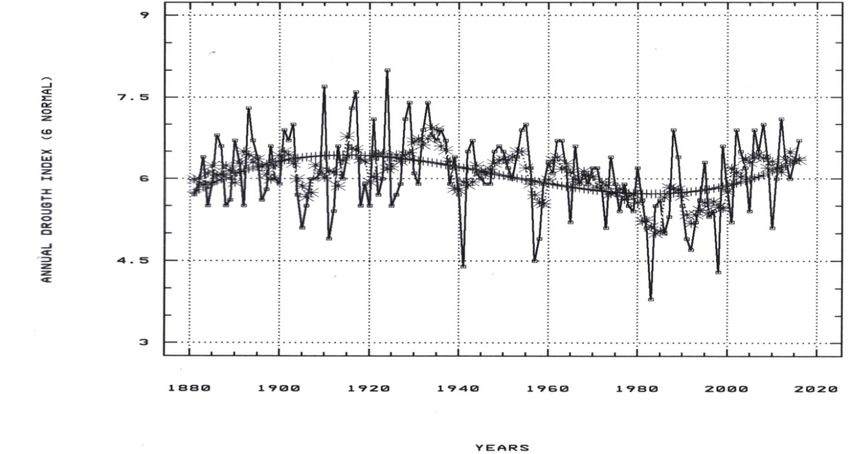
2                             R EVISTA DE C LIMATOLOGÍA , VOL . 19 (2019)

1. Introduction
The intertropical and continental mid-latitude regions of the planet are the main sources of water and
food. These have been the subject of abundant studies for the economic impact and maintenance of
human society, allegedly affected by the Global Warming (GW), IPCC (2001). According to the Basaure
(2007) Earth’s surface is 510 million square kilometers, which 70.7% are covered by water. 30% of the
Earth’s surface of the mainland is cultivated in 9.3%. From this area, USA and India together, cultivate
23% of the total surface in this activity, followed by Russia and China. Among these four countries, the
agricultural area is 40% of the total. Although it is true that most of the crops are located on medium
latitudes, many of them are in the periphery of humid or semi-arid subtropical climate regions affected
by persistent droughts in open expansion observed by their tendencies.
Motivated by the possible impact of the GW on rainfall and other variables, researchers like Chen et al.
(2002) justified the possibility of an intensification of the global convective Circulation of Hadley (CH).
This would be drying the subtropical band and growing in volume to the precipitation of the Equatorial
zone or the Intertropical Convergence Zone (ITCZ). With empirical data of precipitation for the Southern
Hemisphere (SH), Minetti et al. (2014a) warned about the intensification of droughts in Chile Central
(CHI) (Quintana and Aceituno, 2012). Also, making use of climate models, Dai (2013) showed that
the GW would generate an increase in droughts over the subtropical region, enhanced by an increase
in the evapotranspiration and the water deficit. Other researchers have worked with the hypothesis of a
strengthening of CH, expansion of the subtropical anticyclonic zone and shift towards higher latitudes of
the same with the years (Quan et al., 2004, Hu and Fu, 2007; Mitas and Clement, 2005; Minetti et al.,
2009).
This last hypothesis would collide with the agricultural technologists who are increasing the production
surface in the marginal semiarid regions of the Humid Pampas in Argentina, USA, Europe, Australia and
South of Africa among others (Minetti and Sierra, 1984; Minetti et al., 2007). These humid bands of the
world with climate C-Koeppen (1948) have arid BW and semi-arid zones BS (of Koeppen) adjoining,
that exert a natural pressure on them, and by the transitive character on the levels of agricultural produc-
tivity (yields in kg/ha), and also on climate derivatives (Mussio, 2009). This pressure is also increased by
anthropic action with the use of modern technological resources for its purposes (Houghton, 1994, Reb-
oratti, 2010). The same would also be true of tropical climates A-Koeppen either because of an increase
in the frequency of droughts or as an increase in the rate of evaporation of natural ecosystems (Marengo,
2009). Much of the world’s agricultural production is generated in subtropical regions where in recent
decades, intense droughts have been observed in space-time generating a severe and transitory impact
on international grain prices (Ferrelli, 2012; Ortega Gaucin, 2014; Moreno Muñoz, 2010; among others)
putting society at risk of food insecurity (Viñas, 2011). The opposite condition generating storms with
high volume rainfall in a short time associated with the destruction of communication roads, bridges,
main and secondary roads (municipal or communal) have been observed associated with extreme circu-
lation of moisture from the ocean to the continent (external water cycle) and the generation of severe
group or regional-scale monsoon storms in Asia or South America (Minetti et al., 2014b; Minetti, 2005;
Minetti et al., 2013).
For now this seems to be a game of interests on a global-regional-local scale where the demographic
expansion (Dovers et al., 1988, Flores de la Peña, 1954) provides a framework of increasingly adverse
environmental conditions or an unsustainable system (Minetti et al., 2007; Viñas, 2011; Moreno Muñoz,
2010). These would also be interrelated with the supply-demand of energy (Munier, 2012) and financial
businesses (Dabat, 2009) that converge towards more complicated scenarios than the current ones. In
general, the idea of complex interactions ended up being described as a path to collapse of society by
ecologists such as Diamond (2006) and its modeling by Motesharrei et al. (2014). Diamond clarifies in
his book that among the five points that generate instabilities favorable to collapse is the GW or Climate
Change (CC), and for a collapse to occur it would take more than one triggering factor among the five
mentioned by him. This is easily understandable if one sees that another of the points of his consideration
R EVISTA DE C LIMATOLOGÍA , VOL . 19 (2019) 3
has to do with a development not harmonious with nature (non-sustainable activity). Due to its spatial
extension, droughts, unlike water excesses within the climate system, are some of the worst triggers of
regional social-economic collapses, and if their expansion is persistent, such as observed in the CHI and
Subtropical zone of the SH (Minetti et al., 2014a), the collapse is unavoidable with low probability of
adaptation and mitigation.
The analysis of regional droughts in the subtropics zone of the Earth shown as trends or low frequency,
and faster or high frequency fluctuations, would be treated by covering regions of high interest in the
generation of food. In all cases it will try to find some connection between the GW and them. Much
of the current empirical climatologically research has been developed since 1948 when the scientific
community generated a new global database in a grid of latitude and longitude (Kalnay et al., 1996),
which was used to obtain regular meteorological information in the time and space, to be able to diagnose
the climatic past and project towards the future the behavior of a planet warming under diverse scenarios
(assumptions). In this case Dai (2013) using models CMIP3, A1B, CMIp5, and RCP4.5, showed the
areas under aridity on Earth increasing over time, under the effect of a GW with a rate of + 20% between
nowadays and the year 2100, with the impact that this would generate.
The recent information from 1948 to the present would not be sufficient to address the study of the GW
and its impact on the geographical space. For this, it has been necessary to build an ad-hoc base of long-
lived and controlled pluviometric data on the subtropical band and some in the middle latitudes (USA).
The latter is due to the interest shown by the agricultural results that occur in this country that has a large
capacity for production and storage (stocks) for foreign trade, setting the prices of food. The first results
obtained by this group show trend of almost stationary annual rainfall in CHI from the late nineteenth
century to 1950-80 and a growth in dry conditions as of that date, coinciding with the intensification of
the GW from 1980. We need to verify the possible impact of the GW on the hydric conditions of the
subtropical region of the Earth. To do this, it was necessary to: a) present regional rainfall trends in the
SH and NH and also collectively, b) regionally analyze the behavior of droughts and c) relate the GW
to the hydrologic conditions of the study area. The hypothesis of this research is that the GW would
negatively impact the pluviometric conditions of the subtropical region, and in a less homogeneous way,
in the NH.
2. Data and methods
The region studied is located between the parallels +/- 40◦ where the energy balance is positive (Barry
and Chorley, 1972). This includes the CH and the ITC as manifestations of large-scale global convec-
tion. Its seasonal irregularities are due to the summer monsoonal circulation (MC). Towards the N and S,
respectively, the domain of the circulation of middle latitudes begins, included in this work as peripheral
circulation. The thermal data treated here correspond to the monthly-annual series compiled and ana-
lyzed globally by NASA (https://data.giss.nasa.gov/gistemp) whose base has been built with information
from the Meteorological Services of the respective countries of the planet. The annual series of this
variable has been related to the annual water rates treated for this analysis in various regions of the planet
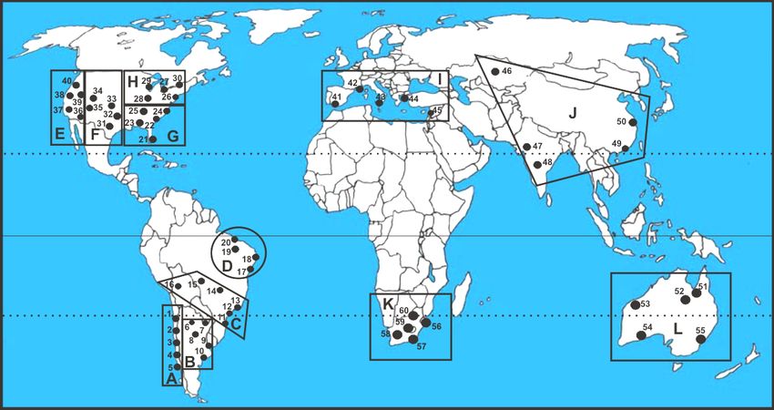
described in figure 1. Locations with monthly rainfall series are shown in table 1. Each region under
analysis has been constructed with around five locations with information (in same case 4 in the NE of
Brazil and 6 in the center of South America), whose water indexes have been estimated with the index
proposed by Minetti et al. (2014a). The monthly drougth index (MDI) is:
MDI = No of dry locations below the medium/No of total locations (1)
with: 0 ≤ MDI ≤ 1 (central value = 0.5)
The annual drought index (ADI) is:
ADI = ∑12
1 MDI (2) with: 0 ≤ ADI ≤ 12 (central value = 6).
The annual drought indexes (ADI) estimated in each region as the percentage of dry locations (referred
to the median central value) over the total of localities in each of the months (1), have some properties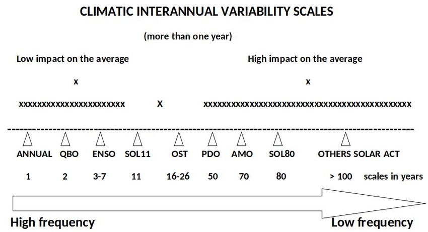
4                             R EVISTA DE C LIMATOLOGÍA , VOL . 19 (2019)

that allow working in situations of lack of data, with at least three locations per area. These indices are
linearly related to the intensity (area-intensity), and their annual value is the sum of the monthly values.
The index is easy to estimate, and the presence of extreme outliers does not affect its temporary treatment
as series, allowing Operational Climate Monitoring. These ADI had been treated as time series for the
purpose of estimating trends. The degree of the polynomial that best fits these series is a complex choice
involving a) the length of the series, b) the presence of medium and long-term climatic phenomena that
are associated with the study of the GW, c) the number of localities analyzed in each region and d) by
other factors.

Fig. 1: Locations with rainfall research on twelve regions of the planet in the period 1880-2016. In each
of the regions there are some rainfall series with data from the period 1850-2016.

                         Table 1: Localities with rainfall information analyzed.

             No    Cities                 Country        Latitude    Longitude     Heigth (m)
              1    La Serena                Chile        29◦ 55’S    71◦ 12’W          28
              2    Santiago de Chile        Chile        33◦ 26’S    70◦ 40’W         564
              3    Concepción               chile        36◦ 46’S    73◦ 03’W          12
              4    Valdivia                 Chile        39◦ 39’S    72◦ 05’W          14
              5    Puerto Montt             Chile        41◦ 26’S    73◦ 05’W          14
              6    S. M. de Tucumán       Argentina      26◦ 51’S    65◦ 06’W         450
              7    Corrientes             Argentina      27◦ 27’S    58◦ 46’W          62
              8    Córdoba                Argentina      31◦ 19’S    64◦ 13’W         474
              9    Buenos Aires           Argentina      34◦ 34’S    58◦ 25’W          6
             10    Bahía Blanca           Argentina      38◦ 44’S    62◦ 10’W          83
             11    Curitiba                Brazil        15◦ 39’S    56◦ 06’W         187
             12    Sao Paulo               Brazil        23◦ 37’S    46◦ 39’W         803
             13    Rio de Janeiro          Brazil        22◦ 49’S    43◦ 15’W          6
             14    Goias                   Brazil        15◦ 55’S    50◦ 08’W         512
             15    Cuiaba                  Brazil        15◦ 39’S    56◦ 06’W         187
             16    La Paz                  Bolivia       16◦ 31’S    68◦ 11’W        4038
             17    Aracaju                 Brazil        10◦ 55’S    37◦ 03’W          5
             18    Maceió                  Brazil        09◦ 31’S    35◦ 47’W         117
             19    Quixeramobim            Brazil        05◦ 12’S    39◦ 18’W         212
             20    Fortaleza               Brazil        03◦ 37’S    38◦ 32’W          25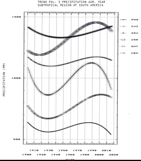
R EVISTA DE C LIMATOLOGÍA , VOL . 19 (2019)                                    5

             No    Cities                   Country        Latitude     Longitude     Heigth (m)
             21    Key West                    US          24◦ 33’N     81◦ 47’W          4
             22    Charleston                  US          38◦ 22’N     81◦ 36’W         299
             23    Mobile                      US          40◦ 31’N     88◦ 15’W          67
             24    Cape Hatteras               US          35◦ 16’N     75◦ 33’W          3
             25    Nashville                   US          36◦ 14’N     86◦ 33’W         173
             26    Whashington                 US          38◦ 58’N     77◦ 27’W          98
             27    Toronto                  Canadá         43◦ 37’N     79◦ 23’W          76
             28    Cincinnati                  US          39◦ 03’N     84◦ 40’W         267
             29    Chicago                     US          41◦ 59’N     89◦ 54’W         205
             30    Burlingston                 US          44◦ 28’N     73◦ 09’W         104
             31    Abilene                     US          32◦ 25’N     99◦ 41’W         546
             32    Little Rock                 US          34◦ 50’N     92◦ 15’W         173
             33    North Platte                US          41◦ 07’N     100◦ 42’W        848
             34    Salt Lake City              US          40◦ 46’N     111◦ 57’W       1289
             35    Phoenix                     US          33◦ 26’N     112◦ 01’W        337
             36    Yuma                        US          32◦ 39’N     114◦ 36’W         34
             37    San Diego                   US          32◦ 44’N     117◦ 10’W         9
             38    San Francisco               US          37◦ 37’N     122◦ 23’W         5
             39    Sacramento                  US          38◦ 34’N     121◦ 29’W         8
             40    Red Bluff                   US          40◦ 09’N     112◦ 15’W        108
             41    Gibraltar               Gibraltar       36◦ 09’N     05◦ 20’W         426
             42    Marignane                 France        43◦ 26’N      05◦ 12’E         32
             43    Palermo                    Italy        38◦ 10’N      13◦ 05’E         34
             44    Athenas                   Greece        37◦ 55’N      23◦ 55’E         73
             45    Beirut                   Lebanon        33◦ 49’N      35◦ 29’E         19
             46    Astana                 Kazakhstan       51◦ 08’N      72◦ 22’E        350
             47    Ahamabad                   India        23◦ 04’N      72◦ 38’E         56
             48    Bangalore                  India        12◦ 58’N      77◦ 35’E        923
             49    Shangai                   China         31◦ 25’N     121◦ 27’E         9
             50    Hong Kong                 China         22◦ 18’N     113◦ 55’E         7
             51    Cloncurry               Australia       20◦ 39’S     140◦ 30’E        200
             52    Alice Spring            Australia       23◦ 47’S     133◦ 57’E        423
             53    Onslow                  Australia       21◦ 40’S     115◦ 06’E         11
             54    Kalgoorlie              Australia       30◦ 47’S     121◦ 27’E        427
             55    Sydney                  Australia       33◦ 56’S     151◦ 10’E         39
             56    Durban                 South Africa     29◦ 57’S      30◦ 56’E         12
             57    Port Elizabeth         South Africa     33◦ 59’S      25◦ 36’E         58
             58    Cape Town              South Africa     33◦ 58’S      18◦ 36’E         56
             59    Kimberley              South Africa     28◦ 48’S      24◦ 48’E       1196
             60    Johannesburgo          South Africa     26◦ 09’S      28◦ 13’E       1676

2.1. Tendency analysis in drought regional indices
The climate variability’s can be represented as the average state of the atmosphere (X̄), it’s periodic (Xp )
and not periodic (X 0 ) variations, as an additive linear representation (3).
This definition of a single variable can be extended to a set of variables that represent it (R = Precipitation,
T = Temperature, P = Atmospheric pressure, and others). In this way X = X̄ + Xp + X 0 (3)               with:
X: variable under analysis
X̄: average of the variable
6 R EVISTA DE C LIMATOLOGÍA , VOL . 19 (2019) X p: periodic diurnal-annual variations and X 0 : disturbance of any temporal scale. 3. Results and discussion The variable X can represent any variable that describes the climate. The Climate Change (CC) as a product of the GW can be represented by changes in X̄ over the years but also as changes in the variability (s, standard deviation or second order moment) and also its 3rd moment order or bias. Disturbances X 0 in turn can represent the inter annual variations of short (QBO, Naujokat, 1986; ENSO, Ropelewski and Halper, 1987), medium and long term scales (Burroghs, 1992; Hoskins, 2012) (figure 2). To represent the average X̄ we should take into account the levels of variability and stability that each variable presents. It is known that the variable of greater instability of rainfall is the average with respect to temperature, pressure and other variables. Also, short-term variations are more unstable than long-term ones. Also, daily rainfall would be more unstable than monthly and annual rainfall, and precipitation would be the most unstable of all the variables. On the other hand, disturbances over 11 years generate instabilities in the estimates of the decadal averages (Herman and Golberg, 1978). Oscillations of these lengths, such as SOL11, OST (Vargas et al. (2002), PDO (Mantua and Hare, 2002), AMO (Schlesinger and Ramankutty, 1994) and SOL80, would destabilize the average values of the rainfall series, confusing such changes with the CC. From the statistical point of view, to obtain averages of long stable periods with errors less than 5% according to Fisher (1963) it would require about 20 years of data on annual rainfall in humid areas, 35 years in semi-arid regions and 50 years in arid areas (Minetti et al., 1986). Fig. 2: Scales of the interannual climate variability phenomena from 1 to 100 years. Annual Wave; QBO: Quasi Biennial Oscillation; ENSO: El Niño Southern Oscillation; 10 year interest limit of this analysis; Undecenal Activity of Sunspots SOL11; OST: Subtropical Oscillation; PDO: Pacifical Decadal Oscilla- tion; AMO: Atlantic Multidecadal Oscillation; SOL80 Large scale or low frequency solar oscillation. The latter is due to the fact that the variability and bias in the frequency distributions of the annual rainfall data increase while moving from a humid to a dry climatic regime. To study CC, at least twice as many of these lengths would be required if the variable analyzed is annual precipitation (Minetti, 1990) and so on successively. There are few data series that comply with this condition according to NASA (2017). It states that there are no more than 1000 locations on Earth that exceed 100 years of observation. The greater concentration of data is also located on medium and subtropical latitudes while the minors are on
R EVISTA DE C LIMATOLOGÍA , VOL . 19 (2019)                                 7

equatorial and polar latitudes. An analysis of CC on the Earth with its impacts should take into account
all those changes over 10 years in length (as interdecadal variations), which can be evaluated by means of
a spectral analysis of the variance (with cycles / sample length of 0.1 or older), according to Tukey (1950)
(figure 3). The calculation of the explained variances over 10 years would then allow us to understand
the importance of large-scale changes in time and space. In addition to these facts, the spectrum of the
variance allows to understanding if the perturbations in the time series would be persistent or not (white
noise or Markov red, Uriel, 1985), and the length-area of the perturbations by the connection between
both.

Fig. 3: (Left): Regional drought indices in South America with the trend and spectra of variance.
(Center): Idem for regions of North America. (Right): Idem for USA regions.

The regions analyzed have been selected because of their geographic location where the maximum de-
creases and drying of the air occurs and in those regions where the agricultural production of grains is
very prominent to later analyze the levels of impacts. With data from annual drought indexes for the
twelve regions, a correlation matrix has been calculated in order to regionalize, at a macro scale, one or
more homogeneous sub regions to analyze the drying processes with time and space.
Figure 4 shows that the region where the anticyclonic band of both hemispheres develops (SH, NH),
with the regions SAF, CHI and ME, the trends can be represented by polynomials 1, 2 and 3 degree with
different approaches (Sagastume and Fernandez, 1960) (table 2). Seven of these regional series admits
three roots, clearly detecting a dry inter decadal stage and a rainy one with maximum amplitude in the
US SE (Peterson et al., 2013). These stages would be around 68 years with quasi periods of 136 years
surpassing the changes of 80 years due to solar activity (Hoskins, 2012 and Herman and Goldberg, 1978,
among others). The length of such changes would not be feasible for analysis in the instrumental period
because of the short length of the series to be treated (136 years). Changes with mathematical expressions
of linear tendencies (polynomial of 1st.Gr.), quadratic (polynomial of 2nd.Gr.) and cubic (polynomial of
3rd.Gr.) can be seen in table 3, where it was possible to group five types of spatial variability. With the
8                            R EVISTA DE C LIMATOLOGÍA , VOL . 19 (2019)

correlation matrix method of Lund (1969) it was possible to group the similar regions in their interannual
variability of the annual drought index, which would be those of Type F, K, J, L and D. The F type group
six American regions, two from South America and four from the USA. Its main long-term model is a
polynomial of degree 3. The Type K model groups three subtropical regions (SAF, CHI and ME). This
model is represented by polynomial quadratic models. Type J, L and M represent independent changes
not connected with the rest.

Fig. 4: Linear (left), quadratic (center) and cubic (right) trends of annual drought indices in the five
clustered regions.

Table 2: Parameters of the adjustments by trend of 1st , 2nd and 3rd degree in the series of regional
droughts. Those trends that match or exceed the explanation of 10% of the total variance are identified
in bold. The significant correlations with the variability of the global temperature are shown (* with
confidence level equal to or greater than 95%). a and b are the coefficients of the regression lines (1st
degree polynomial). S is the standard deviation, and CV the coefficient of variation (Spiegel, 1969).
S2 ≥ 0.1 is the sum of the variances explained in the spectrum lengths of the variance over 10 years. r is
the correlation coefficient with the temperature anomalies of the planet (1900-2006).

         REGION                %S2     %S2     %S2   a        b       S2 CV (%) S2 ≥ 0.1 r con AT◦ G
                              POL1    POL2    POL3
 CHI- CHILE CENTRAL            22.6    24.5    24.7 5.3    +0.017 2.12       22.3       39       +0.44*
  ARG- ARGENTINA               11.1    11.1    16.2 6.6     -0.011 1.65      21.6       34       -0.32*
  CSA- SUDAMERICA              0.05    0.08    4.8 6.0     -0.0006 0.98      16.5       21       +0.02
       CENTRAL
  NSA- SUDAMERICA             0.005    6.6    6.71   6.1    -0.001   2.98    28.5       47        +0.07
        NORTE
    WUS- WEST US               0.01   0.06    1.6 6.4 +0.0003 1.54 19.3                 20        -0.04
CUS- CONTINENTAL US             0     0.04    0.04 5.9 +0.00005 1.05 17.2               22        -0.04
SEUS- SOUTHEAST US             1.07    3.7    24.5 6.2 -0.003 1.31 19.1                 35        -0.08
NEUS- NORTHEAST US             9.5     9.6    14.9 6.5 -0.008 1.08 17.3                 30       -0.24*
 ME- SOUTH EUROPE              10.5   12.5    13.0 5.6 +0.008 1.14 17.2                 38       +0.32*
   MO- SOUTH ASIA              7.5     7.5    12.9 6.7 -0.005 0.72 13.4                 28       -0.32*
 SAF- SOUTH AFRICA             7.4    13.7    17.5 5.4 +0.007 1.02    17                46       +0.34*
   AUS- AUSTRALIA              4.9     5.1    7.2 6.7 -0.006 1.28     18                28       -0.013
        TYPE F                 6.8     6.8    6.9 6.31 -0.004 0.38 10.2                 37       -0.22*
        TYPE K                 30.9   32.6    32.8 5.39 +0.011 0.64 12.95               48       +0.56*
R EVISTA DE C LIMATOLOGÍA , VOL . 19 (2019) 9
Table 3: Interrelationships between inter-annual variabilities regions (main components) from a correla-
tion matrix (N: 136 data, rc = 0.14-Lund, 1969). Chile (CHI), Argentina (ARG), Centre of South America
(CSA), North of South America (NSA), South of Africa (SAF), Mediterranean Zone (ME), Monsoonal
Zone (MO), Australia (AUS), West of USA (WUS), Continental USA (CUS), Southeast USA (SEUS)
and Northeasth USA (NEUS).
REGIONS CHI ARG CSA NSA SAF ME MO AUS WUS CUS SEUS NEUS
CHI 1 +.19 -.18 -.30 -.23
ARG 1 +.14 -.16 +.14 +.19 +.26
CSA +.14 1 +.33 +.30 +.22
NSA 1 -.14
SAF +.19 1 +.24 -.23 -.18
ME -.16 +.24 1 -.18 -.14
MO -.18 +.14 -.23 -.18 1
AUS -.31 -.14 1
WUS 1 +.31
CUS +.19 +.33 -.14 +.31 1 +.15 +.16
SEUS +.26 +.30 -.18 +.15 1 +.21
NEUS -.23 +.22 -.16 +.21 1
Inter-decadal changes in annual global precipitation over ground stations as anomalies (IPCC, 2001)
have been evaluated by Peterson and Vose (1997), Chen et al. (2002), Adler et al. (2003), Rudolf et
al. (1994), Mitchel and Jones (2005) among others. This information shows that rainfall in the long
term went from drier conditions in the first 50 years of the last century (XX) to a rainer season between
1950 and 1990 and a return to drier conditions after 1990, figure 5. A multiple matrix analysis of these
anomalies can be adjusted acceptably by a polynomial of 3er grade as those presented by type F that
group most of the regional drought indices. The presence of the same types of trends makes it possible to
combine criteria of absolute- relative homogeneity of the series of annual rainfall data according to the
WMO (1966). Other hydrological evidences such as the temporal evolution with the years of the height
of Lake Titicaca (Minetti et al., 2014a), connections with other variables (Minetti et al., 2013, 2014b)
and those of non-instrumental type as impacts presented by Minetti and Vargas (1997), give credit about
the real nature of the phenomenon. Also in figure 5 can be seen in a transect West-East the changes of
the sign of the trend of annual precipitation between the South American coast of the Pacific East (Chile-
negative) with respect to the coast of O. Atlántico (East of Buenos Aires, positive ). The latter remains
positive on Uruguay changing the sign of the waves with respect to the continent. These analyze also
show that there is no 100-year sine wave in these trends as shown by Sierra and Perez (2006), and that
global warming is not correlated with all drought indices in the regions. These non-linear behaviors have
also shown that the start and end dates of the series also affect the trends of analyzes shown by Berbery
et al. (2006).
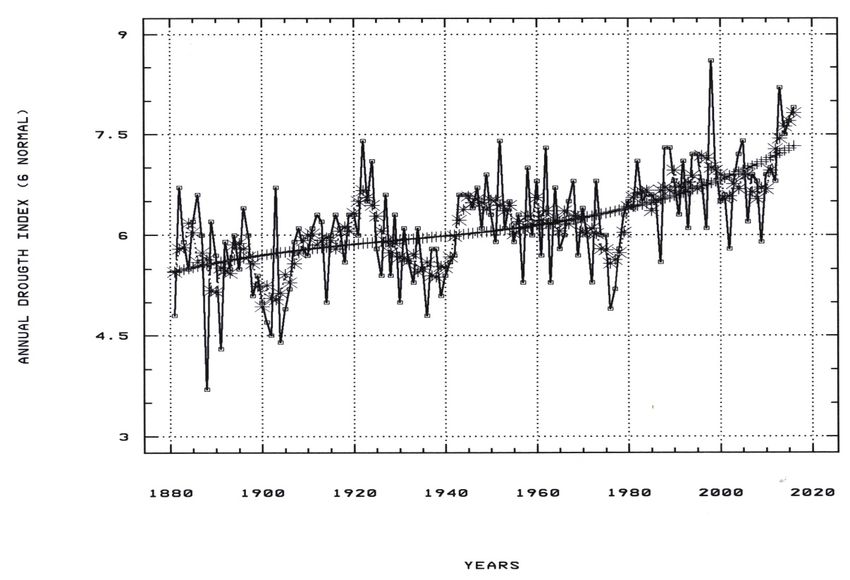
Figure 6 shows the ordinary moving average of 5 years and a trend as a 3er .Gr polynomial, with type
F in order to show that the observed wave is real. These methods excluding the first and last values
because of the methodological limitation of the adjustment In this case, the global series of the IPCC
(2001) covers the period 1900-2006, while in the case analyzed here in this work it covers the period
1880-2016. Inverse series in interdecadal rainy and dry periods can be observed in rainfall for the Sahel-
Central Africa (10◦ -20◦ N, 20◦ W-10◦ E) between 1900-2016 with data from doi: 10.6069 / H5 mW2F2Q
analyzed by Janowiak (1988), confirming the existence of an intensification of HC when forced by the
GW. The long oscillations of the climate are also impacting the SAF in the scales over 10 years with
important quasi-periods of 40 years shown in figure 7 and 8 possibly associated with the Pacific Decade
Oscillation-PDO (Minetti et al. 2010), agreement with (Nicholson and Entekabi, 1986, 1987 a and b,
and 1989). Details of the trends can be seen in the type K model of figures 7 and 8, with intensification10 R EVISTA DE C LIMATOLOGÍA , VOL . 19 (2019) of droughts in the last 40 years apparently forced by the GW. This trend has led to data from the last decade being located within the first decile of the distribution (extraordinary data). The trend is seen through a polynomial adjustment of 3rd. Gr. in types K and F. The opposite condition to type K with a decreasing tendency of droughts or increase in precipitation can be seen in type MO (South of Asia). This case would be explained as the displacement of the CIT towards Asia in the summer (Loo et al., 2015) and the intensification of the convection movements and subsidence in the Subtropics. As subsidence movements of the HC that are evident in CHI, ME and SAF (Philandras et al., 2011). Type L of the NE of Brazil has a reverse connection with the CUS and a parabolic adjustment (figure 4), and turn is inverse to CUS. Type J of AUS (Makuey et al., 2013) is similar to SEUS while maintaining low wave amplitude in contrast to the previous one. Table 4 summarizes the types of variability which have shown significant correlations. Fig. 5: (Above): Trends in annual rainfall in the longest series of southern South America in a North- South transect. (Bottom): Idem in a West-East transect over middle latitudes.
R EVISTA DE C LIMATOLOGÍA , VOL . 19 (2019)                            11

Fig. 6: Annual drought index in types F (first component), and types K (second component). In both
with 3rd degree polinomial tendency and 5 years moving average.

Fig. 7: Annual drought index in the terrestrial subtropics (type K) (second component), trend filtered
with 3rd degree polinomial and 5 years moving average.
12                          R EVISTA DE C LIMATOLOGÍA , VOL . 19 (2019)

Fig. 8: Drought index of types K (CHI, SAF and ME) with 3rd degree polynomial tendency and 5 years
moving average (above). The spectrum of the variance of the index K mode and the correlogram showing
a quasi-periodicity of around 30-40 years (below).

                   Table 4: Types of variability discriminated in the study region.

                 TYPE       Positive correlation Negative correlation
                  F   ARG-CSA-WUS-SEUS-NEUS-CUS         NSA
                  K          SAF-CHI-MED                MO
                   J                AU                CHI-ME
                  L                NSA                  CUS
                  M                 MO            SAF-CHI-MED
R EVISTA DE C LIMATOLOGÍA , VOL . 19 (2019) 13 4. Conclusions The subtropical region of the planet shown in the areas SAF, CHI and ME an increase in the drought indices as positive trends maintained in the last 50 years. The index composed of the three regions, SAF, CHI and ME has a significant correlation with the (GW) and this phenomenon would be due to an intensification of HC. Geographical inhomogeneity between the continental and maritime hemispheres (North-South) and the orographic (East-West) would be responsible for the global irregularity of the HC. Asian monsoonal circulation has a negative trend in annual drought rates, because ITC interrupts CH in South Asia. In this case can see a negative trend (more rainy with the decades), and grow inter annual with major episodes of drought and rainfall. In the SEUS, a trend change is highlighted (3er degree polynomial). It highlights the contrast between the dry period that includes the First and Second World War (1910-1950) with subsequent increase in rainfall between 1950-1990 (rainiest). The trends towards droughts are returning to the last two decades (1995-2016) including the occurrence of severe dry episodes that were also observed in the continental area of South America between the years 2008 and 2013. It is very evident the opposition of signs between the annual rainfall trends between the Pacific and Atlantic coast in mid latitudes of South America and the wave inversion between the continent and the East of the subcontinent. The annual drought indexes are significantly correlated with inter-annual changes in global temperature in the areas of CHI, SAF, ME, and MO, the latter with an inverted sign as it represents the ITC. However it cannot be argued that this effect is anthropic due to the scales involved in the phenomena. The K-type index filtered by 3er degree polynomial shows a quasi-periodic oscillation of almost 40 years, very useful for long-term seasonal climate prediction. Acknowledgments To the National Meteorological Services of each country source of the original data. Institutions that compiled and processed climatological data (Smithsonian Institution and NOAA-USA). To the South American Climatological Laboratory that facilitated the assembly of the database for the analysis and necessary equipment. To Matias A. Minetti for the translations. References Adler RF, Huffman GJ, Chang A, Ferraro R, Xie PP, Janowiak J, Rudolf B, Schneider U, Curtis S, Bolvin D, Gruber A, Sussking J, Arkin P, Nelkin E (2003): The version-2 global precipitation climatology project (GPCP) monthly precipitation analysis (1979-present). Journal of hydrometeorology, 4:1147- 1167. Barry RG, Chorley RJ (1972): Atmósfera tiempo y clima. Ediciones Omega S.A., 395 pgs. Basaure P (2007): Tierras de cultivo a nivel mundial. http://manual de lombricultura.com/foro/dat.pl Berbery EH, Doyle M, Barros V (2006): Tendencias regionales en la precipitación. En: El cambio climático en la cuenca del plata, pp. 67-79. Ed. Barros, Clarke y Dias. Bs. As. Burroughs WJ (1992): Weather cycles real o imaginary? Cambridge Univ. Press, 201 pp.
14                           R EVISTA DE C LIMATOLOGÍA , VOL . 19 (2019)

Chen JY, Clarson BE, Genio AD (2002): Evidence for strengthening for the tropical general circulation
in the 1990s. Science, 295:838-841.
Dabat A (2009): La crisis financiera en Estados Unidos y sus consecuencias internacionales. Problemas
del desarrollo, 40:39-74.
Dai A (2013): Increasing drought under global warming in observations and models. Nature Climate
Change, 3:52-58.
Diamond J (2006): Colapso. Ed. Debate, 747 pp.
Dovers S, Hutchinson F, Buzzard S (1988): Sustainability: definitions, clarifications and contexts. No.
E10 B662d, BIFAD, Washington, DC (EUA).
Ferrelli F (2012): La sequía 2008-2009 en el Sudoeste de la provincia de Buenos Aires (Argentina).
Ecosistemas, 21:235- 238.
Fisher RA (1963): Statistical Methods for Research Workers. Hafner Publishing Co., N. York.
Flores de la Peña H (1954): Crecimiento demográfico, desarrollo agrícola y desarrollo económico. In-
vestigación Económica, 14:519-536.
Herman JR, Goldberg RA (1978): Sun Weather and Climate. NASA, W.D.C. 360 pp.
Janowiak JL (1988): An investigation of interanual rainfall variability in África. J. Climate, 1:240-255.
Houghton RA (1994): The world wide extent of land-use change. BioScience, 44:305-313.
Hoskins B (2012): Escalas de la variabilidad climática interanual. Boletín de la WMO, 61 (1).
Hu Y, Fu Q (2007): Observed poleward expansión of the Hadley circulation since 1979. Atm. Chem.
Phys., 7:5229-5236.
IPCC (2001): Climate Change 2001. Synthesis Report, 397 pp.
Kalnay E, Kanamitsu M, Kistler R, Collins W, Deaven D, Gandin L, Zhu Y (1996): The NCEP/NCAR
40-year reanalysis project. Bull. of the Am. Met. Soc., 77:437-471.
Koeppen W (1948): Climatología. Gráfica Panamericana, 478 pp.
Loo Y, Billa L, Singh A (2015): Effect of climate change on seasonal monsoon in Asia and its impacto
in the variability of monsoon rainfall in Southeast Asia. Geoscience Frontiers, 6:817-823.
Lund IA (1969): Map classification by statistical methods. Journal of Applied Meteorology, 2:56-65.
Makuey G, Mc Arthur L, Kuleshov Y (2013): Analysis of trends in temperatura and rainfall in selected
regions of Australia over the last 100 years. 20th International Congress on Modelling and Simulation,
Adelaide, Australia, 1-6 December.
Mantua NJ, Hare SR (2002): The Pacific Decadal Oscillation. J. Ocean., 58:35-44.
Marengo JA (2009): Long-term trends and cycles in the hydrometeorology of the Amazon basin since
the late 1920s. Hydrol. Process, DOI 10.1002/hyp. 7396.
Minetti JL, Sierra E (1984): Expansión de la frontera agrícola en Tucumán y el diagnóstico climático.
RIAT, 61:109-116.
Minetti JL, Barbieri PM, Carletto MC, Poblete AG, Sierra EM (1986): El régimen de precipitaciones de
San Juan y su entorno. Informe técnico no 8, CIRSAJ-CONICET, San Juan.
Minetti JL (1990): Régimen de variabilidad de las precipitaciones anuales en el Este de Tucumán. RIAT,
67:79-97.
R EVISTA DE C LIMATOLOGÍA , VOL . 19 (2019)                            15

Minetti JL, Vargas WM (1997): Trends and jumps in the anual precipitation in South America, south of
the 15◦ S. Atmósfera, 11:205-221.
Minetti JL (2005): El clima del Noroeste Argentino. Ed. Magna, 449 pp.
Minetti JL, Vargas WM, Vega B, Costa MC (2007): Las sequías en la Pampa Húmeda: Impacto en la
productividad del maíz. Revista Brasileira de Meteorología, 22:218-232.
Minetti JL, Vargas WM, Poblete AG, Mendoza EA (2009): Latitudinal positioning of the subtropical
anticyclone along the Chilean coast. Australian Meteorological and Oceanographic Journal, 58:107-
117.
Minetti JL, Vargas WM, Poblete AG, Bobba ME (2010): Regional drought in the southern of South
America: physical aspects. Revista Brasileira de Meteorologia, 25:88-102.
Minetti JL y otros (2013): El clima de Bolivia. Ed. Minetti. 307 pp.
Minetti JL, Poblete AG, Vargas WM, Ovejero DP (2014a): Trends of the drougth índices in southern
hemisphere subtropical regions. Journal of Earth Science Research, 2:36-47.
Minetti JL, Poblete AG, Vargas WM, Ovejero DP (2014b): Saltos climáticos en el Cuasi Monzón Su-
damericano. Breves Contribuciones del Instituto de Estudios Geográficos, 25:36-57. UNT. San Miguel
de Tucumán.
Mitas C, Clement A (2005): Has the Hadley cell been strengthening in recent decades?. Geophys. Res.
Lett., 32, doi:10.1029/2004GL0211765.
Mitchell TD, Jones PD (2005): An improved method of constructing a database of monthly climate
observations and associated high resolution grids. Int. Jour. of Clim., 25:693-712.
Motesharrei S, Rivas J, Kalnay E (2014): Human and nature dynamics (HANDY): Modeling inequality
and use of resources in the collapse or sustainability of societies. Ecological Economics, 101:90-102.
Moreno Muñoz M (2010): Justicia global y seguridad humana en el contexto del Cambio Climático.
Isegoría, 43:589-604.
Munier BR (2012): Global Uncertainty and the Volatility of Agricultural Commodities Prices. IOS
Press, Doi:10.3233/978-1-61499-037-6-111.
Mussio V (2009): Derivados Climáticos Aplicados a la Agricultura. Universidad Nacional de Rosario,
Argentina.
Naujokat B (1986): An Update of the Observed Quasi-Bienal Oscillation of the Stratospheric Winds
over the Tropics. J. Atm. Sci., 43:1873-1877.
NASA (2017): Anomalías térmicas globales por mes y año. https://data.giss.nasa.gov/gistemp
Nicholson SE, Entekabi D (1986): The quasi-periodic behaviour of rainfall variability in África and its
relationship to the Southern Oscillation. Archives for Meteoro. Geophys and Bioclim., Ser. A, 34:311-
348.
Nicholson SE, Entekabi D (1987a): African enviromental and climatic changues and the general atmo-
spheric circulation in late Pleistocene and Holocene. Climate Change, 2:313-348.
Nicholson SE, Entekabi D (1987b): Rainfall variability in equatorial and Southern África: Relationships
with sea-surface temperatures along the southwerstern coast of Africa. J. Climate and Appl. Meteorol.,
26:561-578.
Nicholson SE (1989): Long-Term changes in African rainfall. Weather, 44:46-56.
16                           R EVISTA DE C LIMATOLOGÍA , VOL . 19 (2019)

Ortega Gaucin D (2014): Sequía en México y Estados Unidos de América: diferencias esenciales de
vulnerabilidad y enfoques en la atención al fenómeno. Frontera Norte, 26:141-148.
Peterson TC, Vose RS (1997): An overview of the Global Historical Climatology Network temperature
database. Bull. of the Am. Met. Soc., 78:2837-2849.
Peterson TC, Heim RR, Hirsch R, Kaiser DP, Brooks H, Diffenbaugh NS, Dole RM, Giovannettone
JP, Guirguis K, Karl TR, Katz RW, Kunkel K, Lettenmaier D, McCabe GJ, Paciorek CJ, Ryberg KR,
Schubert S, Silva VB, Stewar BC, Vecchia AV, Villarini G, Vose RS, Walsh J, Wehner M, Wolock D,
Wolter K, Woodhose CA, Wuebbles D (2013): Monitoring and understanding changes in heat waves,
cold waves, floods, and droughts in the United States. State of Knowledge. Bull. Am. Met. Soc.,
94:821-834.
Philandras CM, Nastos PT, Kapsomenakis J, Douvis KC, Tselioudis G, Zerefos CS (2011): Long term
precipitation trends and variability within the Mediterranean región. Natural Hazards and Earth System
Sciences, 11:3235-3250.
Quan XW, Diaz HF, Hoerling MP (2004): Change of the tropical Hadley cell since 1950. In: The Hadley
circulation: present, past and future, pp. 85-120, Springer.
Quintana JM, Aceituno P (2012): Changes in the rainfall regime along the extratropical west coast of
South America (Chile): 30-43◦ S. Atmósfera, 25:1-13.
Reboratti C (2010): Un mar de soja: la nueva agricultura en Argentina y sus consecuencias. Revista de
geografía Norte Grande, 45:63-76.
Ropelewski CF, Halper MS (1987): Global and regional scale precipitation and temperatura patterns
associated with El Niño/Southern Oscillation. Mon. Wea. Rev., 115:1606-1626.
Rudolf B, Hauschild H, Rueth W, Schneider U (1994): Terrestrial precipitation analysis: Operational
method and required density of point measurements. In: Global Precipitations and Climate Change, pp.
173-186. Springer Berlin Heidelberg.
Schlesinger ME, Ramankutty N (1994): An oscillation in the global climate system of period 65-70
years. Nature, 367:723-726, DOI:10.1038/367723a0.
Sagastume Berra AE, Fernández G (1960): Álgebra y Cálculo Numérico. Ed. Kapeluz, 726 pp. Bs. As.
Sierra EM, Perez SP (2006): Tendencias del régimen de precipitación y el manejo sustentable de los
agroecosistemas: estudio de un caso en el noroeste de la provincia de Buenos Aires, Argentina. Rev.
Climatol., 6:1-12.
Spiegel MR (1969): Estadística. Mc Graw-Hill, Panamá, 357 pp.
Tukey JW (1950): The sampling theory of power spectrum estimates. Symposium on Applications of
Autocorrelation Analysis to Physical Problems. U.S. Office of Naval Research. NAVEXOS. P735, 47-
67. Washington, DC.
Uriel Jimenez E (1985): Análisis series temporales. Modelos ARIMA. Paraninfo SA. 270 pp., Madrid.
Vargas WM, Minetti JL, Poblete AG (2002): Low-frequency oscillation in climaticand hydrological
variables in southern South America’s tropical-subtropical regions. Teor. Appl. Clim., 75:1-12.
Viñas JMS (2011): Volatilidad de los mercados agrarios y crisis alimentaria. Revista española de estudios
agrosociales y pesqueros, 229:11-35.
Word Meteorological Organization (WMO) (1966): Climatic Change. Technical Note No 79, Geneve.
You can also read