Trip generation modeling for a selected sector in Baghdad city using the artificial neural network
←
→
Page content transcription
If your browser does not render page correctly, please read the page content below
Journal of Intelligent Systems 2022; 31: 356–369 Research Article Safa Ali Lafta* and Mohammed Qadir Ismael Trip generation modeling for a selected sector in Baghdad city using the artificial neural network https://doi.org/10.1515/jisys-2022-0023 received September 25, 2021; accepted November 04, 2021 Abstract: This study is planned with the aim of constructing models that can be used to forecast trip production in the Al-Karada region in Baghdad city incorporating the socioeconomic features, through the use of various statistical approaches to the modeling of trip generation, such as artificial neural network (ANN) and multiple linear regression (MLR). The research region was split into 11 zones to accomplish the study aim. Forms were issued based on the needed sample size of 1,170. Only 1,050 forms with responses were received, giving a response rate of 89.74% for the research region. The collected data were processed using the ANN technique in MATLAB v20. The same database was utilized to develop the model of multiple linear regression (MLR) with the stepwise regression technique in the SPSS v25 software. The results indicate that the model of trip generation is related to family size and composition, gender, students’ number in the family, workers’ number in the family, and car ownership. The ANN prediction model is more accurate than the MLR predicted model: the average accuracy (AA) was 83.72% in the ANN model but only 72.46% in the MLR model. Keywords: trip production, artificial neural network, multiple linear regression, household, modeling 1 Introduction Urban transport is a multidimensional concept and a part of metropolitan mobility that combines the movement of merchandise, inhabitants, and information between urban regions [1]. Transportation is defined to be the movement of people, goods, and services from one place to another during a desirable condition, whereas transport planning is interested in the development of a plan with respect to the economic, social, and environmental effects of the populace to enhance the positive objectives. The funda- mental aim of transportation planning is to accommodate the requirement for mobility in order to provide effective access to different activities that satisfy human needs. These reasons make it important to prepare comprehensive analyses of the regions in order to establish the origins of these journeys and then deter- mine the origin and destination of these journeys in order to create statistical models to forecast the movement of these journeys. Therefore, recent studies have concentrated on the transportation system’s appropriateness and robustness, as well as future demand [2]. Trip demand refers to the group of individ- uals or vehicles that could be expected to move on a given section of a transportation network during a given time span, based on land use, social, economic, and environmental variables. Forecasting of trip demand estimates the number, type, and origin of “trips” (source and target) on the transportation network * Corresponding author: Safa Ali Lafta, Department of Civil Engineering, College of Engineering, University of Baghdad, Baghdad, Iraq, e-mail: s.alshatawi1901m@coeng.uobaghdad.edu.iq Mohammed Qadir Ismael: Department of Civil Engineering, College of Engineering, University of Baghdad, Baghdad, Iraq, e-mail: drmohammedismael@coeng.uobaghdad.edu.iq Open Access. © 2022 Safa Ali Lafta and Mohammed Qadir Ismael, published by De Gruyter. This work is licensed under the Creative Commons Attribution 4.0 International License.
Trip generation modeling for a selected sector in Baghdad using ANN 357
[3]. The problem of urban transportation is caused by a number of interrelated causes. The high urban
population growth and real expansion in urban areas as a result of population redistribution, improved
living conditions due to higher incomes, and consequently the increased dependence on private automo-
biles are just some of these reasons [4]. A well-established transport system’s important criterion is the
anticipation and availability of transport services [5,6]. In addition, the implementation of comprehensive
transportation planning may help minimize the difficulties that could arise in the future and pave the way
for a sustainable urban transportation system [7].
The modeling of travel demand plays a basic role in the planning of effective transport networks as it
offers useful data on traveler preferences and predicts current and future demand for travel within a
rational context. Travel demand is defined as the number of individuals or automobiles that may be
expected to utilize a segment of a transport system during a specific amount of time within a variety of
different environmental, economic, social, and land usage circumstances. The forecast for travel demand
anticipates the number, kind, and source of journeys on a transport network [3]. Numerous studies have
been conducted on the relationship between urban transport and passenger travel demand. Research
studies have documented the influence of land usage and the built environment on trip production and
trip production by activity and intent, journey frequency, selection of location, geographic scale selection,
and mode choice [8]. The demand for a metropolitan center in an area relies on the relative accessibility,
connectedness, and appropriateness of transportation [6]. In specific, the four-step forecasting method for
travel demand, known as the urban transport modeling system, Typically, this method transfers metropol-
itan activities into many journeys and aims to estimate the relation between metropolitan activities and
travel via modeling trip generation, distribution of trips, selection of mode, and assignment of traffic. The
first stage in the traffic demand forecasting process is trip generation prediction. The aim of the generation
stage of the trips is to recognize the causes that explain the behavior of travel patterns and to create
statistical models to synthesize the travel behavior, according to the information of travel survey, land
use, and characteristics of the household. Conventionally, trip generation predictions are established
independently of any straight consideration of the transportation network. This means that trips produced
in or attracted to a zone are a function only of the characteristics of the zone itself and are not specifically a
function of the transportation network on which the travels are made [4]. The rising population and
geographic development of cities improve urban public transportation accessibility [9]. As public trans-
portation is likely to make metropolitan districts more accessible and sustainable, improving public trans-
portation accessibility may be considered a primary goal of transportation development. A more efficient
transportation system lowers transaction costs, allows economies of scale and specialization, extends
options, improves commerce, consolidates marketing, and increases society’s income and welfare [10].
Hypothetically, developing a model from an empirical dataset is not always achievable. There are various
causes for this, including the presence of nonlinearity and/or colinearity between parameters, as well as the fact
that sometimes building a model is simply too hard. As a result, the methodology of the artificial neural
networks (ANNs) is a critical component of model development, data analysis and assessment, and prediction
independent of statistical approaches [11]. Therein, information can be simulated in order to develop an optimal
model that explains the phenomenon that can be employed in the majority of cases and circumstances.
The use of neural networks in statistics has the following contributions:
• The approach is seen as a modern data analysis pattern in which patterns are not specified directly but
rather defined implicitly by the network.
• It provides advanced model recognition capabilities.
• It allows for analysis in circumstances wherein conventional methods might be incredibly tedious or
nearly difficult to interpret.
Multiple linear regression (MLR) is commonly used in trip generation modeling, and it has specific
conditions. Alternative modeling techniques with less stringent conditions are required if the conditions for
employing MLR are not met, The ANN method is model free. This is a method that is based on data. ANN
does not make strict model suppositions such as normality, linearity, or mutual independence of autono-
mous variables. This is why ANN might be more advantageous for trip generation modeling. To improve the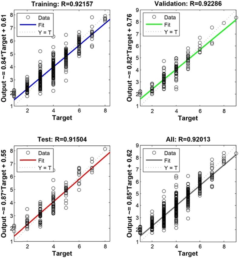
358 Safa Ali Lafta and Mohammed Qadir Ismael
efficiency of the predicted model, ANN models must be developed in a systematic manner. In this study, the
same database utilized to develop the model of multiple regression was utilized to develop a multilayer
feed-forward back-propagation ANN model using a neural network tool in the MATLAB v20 software
because MATLAB allows nonexperts to develop neural networks.
2 Literature review
Al-Hasani, developed relationships between daily trips and socioeconomic characteristics for the Al-Karkh
region of Baghdad city [12]. The research area was split into 10 zones. The equation of trip generation was
obtained using both MLR and cross-classification techniques. According to the findings, the overall trip per
person per household is linked to the size of the family and variables of structure, such as the number of
people above the age of 6, the number of males, and the number of male workers. It also is related to the
availability of cars and the kind of housing unit. For all research regions, a model with a coefficient of
determination (R2) of 0.678 was developed [12].
Naser and Mahdi utilized ANNs to model trip generation in their research on the initial stage of transport
planning [13]. The research evaluated the effectiveness of ANNs using data obtained for the city of Nasiriyah
central business district by calculating all trips (y) generated by this sector. As a consequence, the ANN model
outperformed statistical techniques in forecasting trips. The coefficient of determination R2 for the total number
of trips (y) was 0.948 for the ANN and 0.871 for the statistical technique approaches, which is regarded as an
acceptable relationship; moreover, the ANN prediction model is more accurate for the prediction process [13].
Peng et al. focused on integrating neural networks that had excellent fitting ability and the genetic
algorithm’s excellent global searchability with the trip generation prediction model in order to enhance
prediction accuracy, and they designed two types of trip generation prediction models based on genetic
algorithms and neural networks [14]. Thus, there is much work to be done in this area. In a nutshell,
integrating genetic algorithms and neural networks with transportation prediction is one method toward
precise and rational traffic planning and design [14].
In recent years, transport planners have increasingly used neural networks to develop transportation
models, particularly trip demand models. Over the last decade, a growing amount of literature has exam-
ined the efficiency of neural network techniques for estimating and analyzing travel demand [15].
The back-propagation ANN model outperforms the multiple regression model in terms of trip genera-
tion prediction as demonstrated by the R2 value in previous research studies. In this study, the collected
data from the field was processed using multilayer feed-forward neural networks by MATLAB v20, and it
was more flexible than SPSS because the latter might not provide the required results be due to the type of
training algorithm that was used.
3 Research objectives
Transport network is considered a major infrastructure, and it represents the degree of development in the
area. The number of vehicles has increased more than two fold after 2003 in Baghdad according to the
Traffic Police Directorate. The land usage in several sectors has changed, and expansion of residential areas
is noticeable in other sectors. As a result, performing the daily activities has become a burden that grows
with each passing day. The process is intended to create a statistical prediction model that explains the
behavior and the relationship of the considered hypothesis. Therefore, the main aim of the research is to
determine the pattern of household travel characteristics in the research region and to develop statistical
models for a trip generation. The specific objectives are as follows:
• Obtain accurate and detailed data on household travel characteristics wherever possible in the Al-Karada
region of Baghdad urban area
• Develop models for trip generation using the ANN technique and the MLR technique for building the models.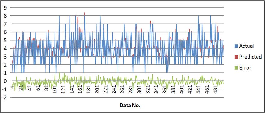
Trip generation modeling for a selected sector in Baghdad using ANN 359
3.1 Research methodology
Data collection is critical and one of the most challenging stages in the urban transit process. It requires
comprehensive investigation, extensive planning, qualified interviewers, cost, and time, as well as some
governmental assistance. The methodology of the research for data collection should be accomplished with
a sequence of steps in order to avoid flustering [16]. The following steps are appropriate to be followed:
3.2 The study area zoning
To simplify the collection of data in the transportation planning process, the research region is divided into
a set of zones that are subdivided to assist in geographically connecting the origin and destination of the
trip. Zones within the outermost cordon of the study area are known as internal zones whereas the others
are known as external zones [17].
4 Zone coding
Baghdad city was split into 10 sectors. Each sector was split into a series of zones for the objectives of data
collection and surveillance; hence the total number of traffic analysis zones (TAZs) is forty-five. The zoning
is based on the governmental partitions of council municipalities.
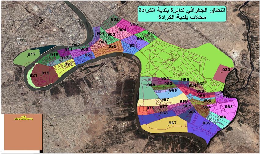
In this study, the region of the study was divided into 11 zones (901, 903, 905, 907, 909, 911, 913, 915,
923, 925, and 929). The zoning was according to the administrative partitions of council municipals, under
which some additional partitions of council municipals (Hay Al-Karada) consist of zones (901, 903, 905,
907, and 909); Hay Al-Jamiea consists of zones (911, 913, and 915); and Hay Babil consists of zones (923, 925,
and 929 as presented in Figure 1. The population and number of households in the TAZs have been
tabulated and presented in Table 1.
Figure 1: TAZ of the study region according to the municipality divisions [Amanat Baghdad].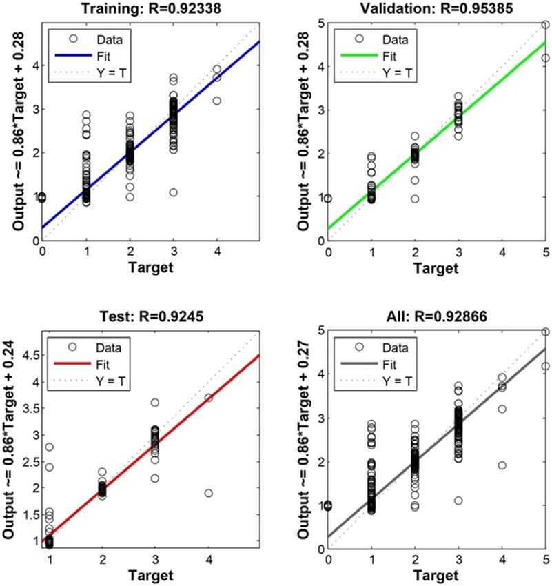
360 Safa Ali Lafta and Mohammed Qadir Ismael
Table 1: Population and number of households in the TAZs according to the municipality divisions
Traffic analysis zone No. of households Population
901 1,689 6,636
903 3,459 14,283
905 2,626 10,682
907 2,140 8,769
909 3,931 14,976
911 1,576 6,629
913 500 2,500
915 2,657 6,382
923 1,211 5,114
925 1,787 6,769
929 1,720 8,600
Total 23,296 91,340
4.1 Sample size
Data are collected in urban transportation planning studies in either of two methods: through the home inter-
views method or through the distribution of questionnaire forms method. It would be important to set the
necessary sample size for both ways. The required sample size to be interviewed is based on the overall
inhabitants living in the research region. Censuses of inhabitants and households are obtained from the research
area’s municipal council for accuracy. In the specified research region, there are 91,340 residents and the
aggregate number of families is 23,296. It is not practical to gather the data from all populations of the research
area. As a result, it became essential to calculate the sample size according to the density of the inhabitants of the
research region and represents the minimum and optimal values for the size of the sample in Table 2 [19].
Table 2: Sample size for home interview survey [18]
Population of study area Sample size
No. of households Population
Under 50,000 1 in 10 1 in 5
50,000–150,000 1 in 20 1 in 8
150,000–300,000 1 in 35 1 in 10
300,000–500,000 1 in 50 1 in 15
500,000–1,000,000 1 in 70 1 in 20
Over 1 million 1 in 100 1 in 25
Note: The population of the study area was between (50,000–150,000) . As a result, the appropriate sample size for the
inhabitants of the research region is 1 in 20.
As presented in Table 2, the appropriate sample size for the inhabitants of the research region is 1 in 20.
As a result, the required sample size is as follows:
Sample size = [1 /20] × 23,296 = 1164.8
As a result, 1,170 questionnaire forms were distributed.
5 Household trip generation modeling
To develop a trip generation model that assumes a relationship between the number of trips produced (the
dependent variable) and the socioeconomic characteristics (the independent variable) in the region under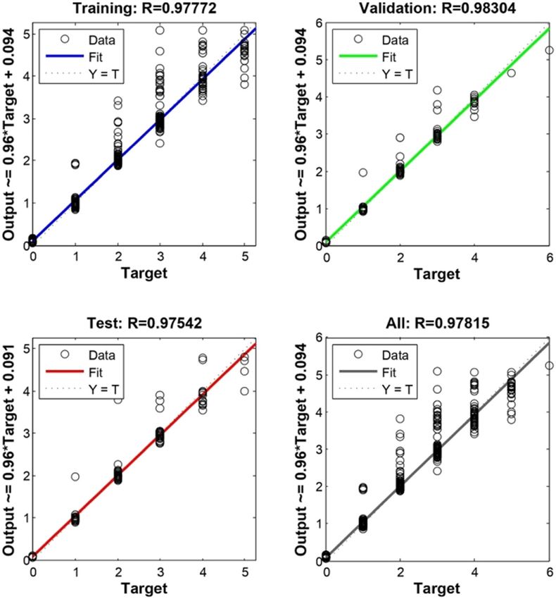
Trip generation modeling for a selected sector in Baghdad using ANN 361 study, for example, mean value income, car ownership, number of families, and so on, ANN and MLR were adopted to develop the model. The following variables were included in the analysis: 1. Dependent variables: • Y: Household overall trips type/day • Y1: Household work trips/day • Y2: Household educational trips/day • Y3: Household shopping trips/day • Y4: Household social trips/day • Y5: Household other trips/day 2. Independent variables: • X1: Family size (No.) • X2: Number of men in the family (No.) • X3: Number of women in the family (No.) • X4: Number of workers in the family (No.) • X5: Number of students in the family (No.) • X6: Household individuals less than 6 years old (No.) • X7: Household individuals 6–18 years old (No.) • X8: Household individuals 19–24 years old (No.) • X9: Household individuals 25–60 years old (No.) • X10: Household individuals more than 60 years old (No.) • X11: Household monthly income (1, 2, 3) • X12: Dwelling unit type (house, apartment) (1, 2) • X13: Dwelling unit ownership (own, rented) (1, 2) • X14: Area of the dwelling unit in sq. m (1, 2, 3) • X15: Car ownership (No.) 5.1 Development of MLR model The MLR models of trip production were developed via the SPSS v25 software. The stepwise method is the best and commonly used to derive simple prediction regression models for each independent variable [19]. Table 3: Descriptive statistics of independent variables Item Variable Mean Std. deviation X1 Family size 4.813 1.5999 X2 No. of men 2.289 1.173 X3 No. of women 2.528 1.178 X4 No. of workers 1.613 0.667 X5 No. of students 2.199 1.282 X6 Persons less than 6 years 0.481 0.706 X7 Persons 6–18 years 1.480 1.154 X8 Persons 19–24 years 0.809 0.762 X9 Persons 25–60 years 1.762 0.688 X10 Persons more than 60 years 0.282 0.563 X11 Household income 2.035 0.689 X12 Dwelling unit type 1.149 0.357 X13 Dwelling unit owner 1.281 0.450 X14 Dwelling unit area 1.434 0.535 X15 No. of car owners 0.760 0.545
362 Safa Ali Lafta and Mohammed Qadir Ismael
Table 4: Stepwise regression model parameters of all production trip types
Trip type Model R2 Adj R2 S.E.E
Work trips (Y1) 0.076 + 0.958X4 + 0.054X15 − 0.034X9 + 0.027X12 + 0.019X1 0.949 0.949 0.144
Educational trips (Y2) 0.145 + 0.860X5 + 0.087X7 − 0.057X1 + 0.064X13 − 0.025X6 0.923 0.923 0.324
Shopping trips (Y3) 0.035 + 0.875X1 + 0.1X4 + 0.035X3 0.842 0.841 0.272
Social trips (Y4) −0.049 + 0.835X1 − 0.139X4 + 0.049X12 + 0.028X15 0.845 0.844 0.256
Other trips (Y5) 0.652 + 0.39X2 + 0.098X15 + 0.102X10 0.871 0.870 0.467
Total trips (Y) 0.469 + 0.770X5 + 0.847X4 + 0.139X15 + 0.127X1 + 0.139X11 − 0.120X8 + 0.851 0.850 0.528
0.055X2
The autonomous variable with the greatest F test score is chosen as the initial entry variable. The operation
continues if at least one parameter exceeds the criterion. The method considers adding a second indepen-
dent variable to improve the model. This evaluates all parameters to see which ones have a test of the
F-value and which ones match the F-test selected for inter criterion. Either F value test or probability of F
value test is used as enter criteria. F is employed as a probability equal to 0.05 in the analysis, and this
coincides with an F test value of 3.48. Table 3 shows the descriptive statistics for autonomous variables that
were utilized in the development of trip production models. Table 4 summarizes the stepwise regression
models with a confidence level of 0.95.
In the model of the total trips, it can be noticed that number of students (X5), worker number (X4),
number of car owners (X15), family size (X1), family income (X11), and the number of men (X2) are the
effective independent variables in the calculation of these trips whereas the parameter of the number of
persons 19–24 years (X8) has a negative effect on these trips.
5.2 Modeling trip generation using ANNs
The database utilized to develop the MLR model was also utilized to develop a multi-layer feed-forward
back-propagation ANN model using a neural network tool in the MATLAB v20 software because MATLAB
allows nonexperts to develop neural networks. Dividing the available data into three sets of training,
validation, and testing to forecast trips in 1,050 observational data sets, a multilayer feed-forward back-
propagation neural network model and sigmoid function were developed. Randomly selected (70%) data
were utilized to train the network and the remaining samples (30%) were evenly divided for ANN validation
and testing operations (selected 15% as test data and used the other 15% for network validation). To
evaluate the validity of the obtained equations for all types of trips (Y), the developed ANN models were
utilized to forecast these values based on all training and validation data sets applied as shown in the
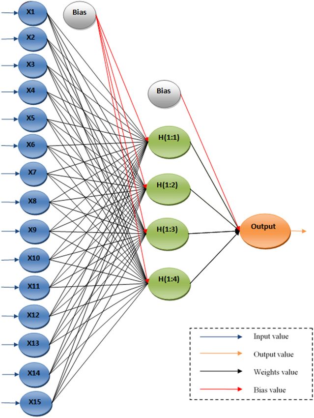
network diagram in Figure 2. The predicted values for all trips (Y) and the projected values are near to actual
values, which indicate that a strong correlation exists between the input and output data, and can also be
seen in Figures 3–8, respectively for the data sets.
An artificial neuron collects x1, x2, …, xn input signals, each of which is assigned a weight (Wik)
indicating the strength of the connections for all connections, which will vary throughout the training
process. The resultant connection weight is multiplied by each input signal. A bias (bk) seems to be a type of
connection weight created by applying a constant nonzero value to the sum of the inputs and the resulting
weights (Ik). The measure of the combined input is transmitted to a preselected transfer or activation
function (T) and generates (Yk) during the transfer function plotting, as the artificial neuron’s outgoing
end (k), as defined in equations (1) and (2).
Ik = ∑WikXi + bk, (1)
Yk = T (I ) , (2)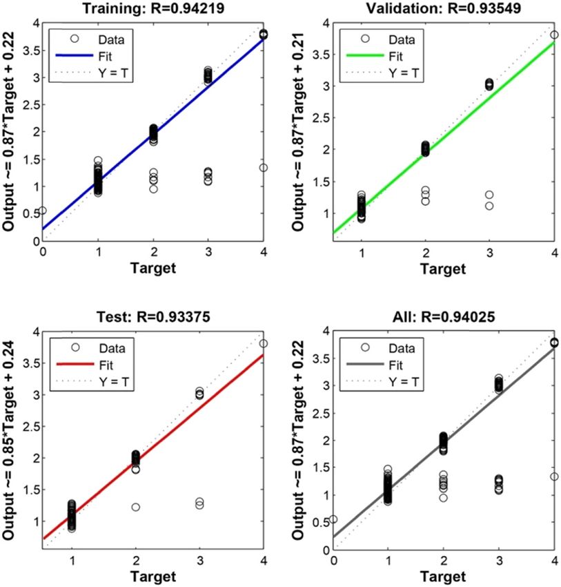
Trip generation modeling for a selected sector in Baghdad using ANN 363
Figure 2: Structure of the ANN optimal model.
where IK – the level of activity of node K; Wik – the weight of the connection among nodes (I) and (k);
Xi – the input of the node (i), where (i = 0, 1, 2, …, n); bk – the bias to node (k); Yk – the output to node (k);
and T(I) – the transfer function.
There are several types of transfer functions in the neural network toolbox. In this study, we used the
most common function in neural networks, the logistic sigmoid function, due to its differentiability.
Equation (3) describes the sigmoid function:
1
T (I ) = , (3)
1 + e−ØI
where ∅ is a positive scaling constant that controls the steepness of the asymptotic range between 0 and 1.
This function builds well-behaved neural networks. The inhibitory and exciting impacts of weight variables
are clearly visible with this feature, which also allows for more efficient network training [20,21].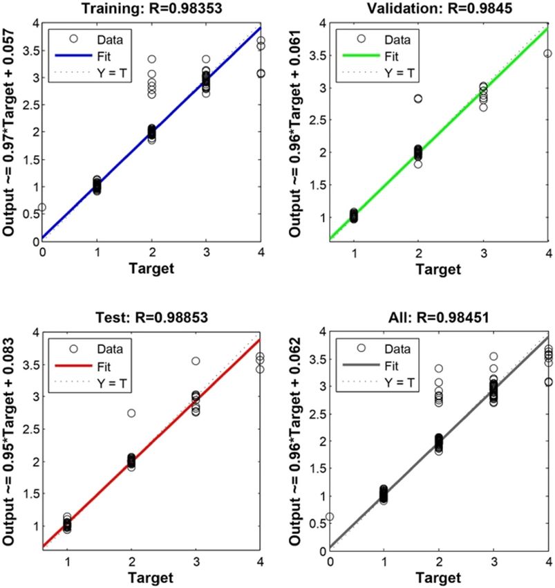
364 Safa Ali Lafta and Mohammed Qadir Ismael
Figure 3: Predicted value compared with the observed value for work trips (Y1).
Figure 4: Predicted value compared with the observed value for educational trips (Y2).
The error percentages of the trip generation for sample data are also shown in Figure 9. Table 5 exhibits
the mean squared error (MSE), the root mean squared error (RMSE), and the coefficient of determination
(R2) values that were developed in this study to assess the relevance of the ANN model.Trip generation modeling for a selected sector in Baghdad using ANN 365
Figure 5: Predicted value compared with the observed value for shopping trips (Y3).
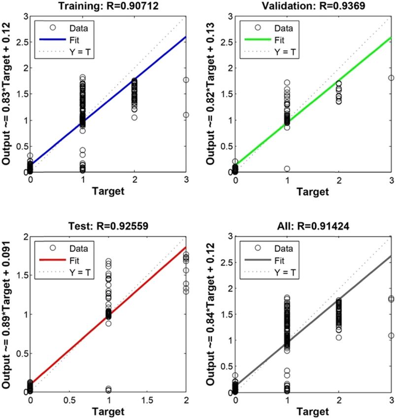
Figure 6: Predicted value compared with the observed value for social trips (Y4).
Weights were determined and adjusted using network training and the data set was split into training
and test information. The weights seized and their performance is summarized in Table 6. Where these
weights are the best weights through, which we can get the best and most accurate results.
The forecast of the trip generation model for the Al-Karada region has been made using both MLR and
ANN methods. A statistical comparison of the performance of the two approaches was made and is366 Safa Ali Lafta and Mohammed Qadir Ismael Figure 7: Predicted value compared with the observed value for other trips (Y5). Figure 8: Predicted value compared with the observed value for all trips (Y). presented in Table 7. Accordingly, the back-propagation ANN model outperforms the MLR model in terms of trip generation prediction, as demonstrated by the greatest R2 value, with R2 for (Y) being 0.851 in MLR as compared with 0.92441 under the ANN technique. In addition, the MSE and RMSE values for the ANN model were lower than for the MLR model. The ANN approach in forecast of the trip production model is better than the MLR approach from the statistical point of view and more accurate, with the average accuracy of
Trip generation modeling for a selected sector in Baghdad using ANN 367
Figure 9: Comparison of actual and predicted values for sample data.
Table 5: Performance of all production trip types in ANN model
Trip type R2 MSE RMSE
Work trips (Y1) 0.98451 0.012206 0.110481
Educational trips (Y2) 0.97815 0.04448 0.210903
Shopping trips (Y3) 0.94025 0.062208 0.249415
Social trips (Y4) 0.91424 0.032764 0.18101
Other trips (Y5) 0.92866 0.067702 0.260196
Total trips (Y) 0.92013 0.24756 0.497554
Table 6: Variables and weights
Weights Hidden layer
H(1:1) H(1:2) H(1:3) H(1:4)
Input layer X1 0.56065 0.18821 −0.7774 0.7678
X2 −0.54803 0.073832 −1.311 0.32863
X3 −0.46374 0.43045 −1.2458 0.174022
X4 1.7867 1.3423 1.1083 0.95888
X5 1.1319 0.70558 1.183 1.2617
X6 −0.048773 −0.49819 0.79076 −0.21212
X7 −0.041639 −0.62261 0.58729 0.063275
X8 0.33032 −0.41309 0.052879 −0.57759
X9 −0.015592 −−0.88548 −0.69552 0.1528
X10 −0.42331 −0.63712 0.5932 −0.4796
X11 −0.88709 −0.76867 1.0326 0.54517
X12 0.2107 −0.5479 −0.0663 0.10948
X13 0.026772 0.93805 1.0907 −0.15009
X14 0.45077 0.34324 −0.70237 0.06358
X15 0.051465 −0.60928 0.43639 0.815969
Biases Hidden layer
Input layer −2.0604 −1.9623 −0.78168 0.8057
Output layer Weights Biases
Hidden layer
H(1:1) H(1:2) H(1:3) H(1:4)
1.8105 −0.63887 0.60004 1.2566 −1.3555368 Safa Ali Lafta and Mohammed Qadir Ismael
Table 7: Statistical comparison among MLR and ANN techniques
Description ANN MLR
R2
0.920 0.851
MSE 0.248 0.279
RMSE 0.498 0.529
MAPE 16.277 27.540
AA% 83.723 72.460
83.72% in the ANN model and 72.46% in the MLR model. The ANN model’s mean absolute percentage error
(MAPE) categorization is superior to that by the MLR model with categorization of 83.72% as against 72.46%
in the latter.
6 Discussion
The essential independent factors that impact the overall trip generation percentage in the study region are
students’ number, workers’ number, the number of car owners, family size, income of the family, and
number of males. A small increase in the monthly household income leads to a slight rise in the average
household journeys for MLR. There is an important relationship between the mode of transportation usage
and monthly household income. Families that have high monthly income have a propensity to utilize
private cars whereas families with low monthly income show a propensity to use public transportation.
7 Conclusion
• The back-propagation ANN model outperforms the MLR model in terms of trip generation prediction, as
demonstrated by the greatest R2 value, with R2 for (Y) being 0.851 in MLR as compared with 0.920 under
the ANN technique. Thus, it can be regarded as a very good prediction model.
• The values of MSE and RMSE for the ANN model were lower than that for the MLR model.
• In comparison with the MLR-predicted model, the ANN-predicted model is more accurate. The average
accuracy (AA) is 83.72% in the ANN model and 72.46% in the MLR model.
• The ANN model’s MAPE categorization is superior to that of the MLR model’s with the categorization of
83.72% as against 72.46% in the latter.
• The ANN method may be utilized for trip production models as it results in less prediction error.
• It is proposed that a zone system for Baghdad be developed and a database for all road networks be
created utilizing a computer program such as geographical information system software for creating the
optimal zoning system.
• ANN can be utilized to develop models for other transport planning stages such as trip distribution, spilt
of modal transport, and traffic assignment for the Al-Karada sector in Baghdad city and other cities
in Iraq.
• Another technique in ANN, namely, fuzzy logic, can also be used in trip production modeling.
Acknowledgments: The authors are grateful to the Civil Engineering Department, College of Engineering,
University of Baghdad, for support and help in accomplishing the work contained in this research.
Conflict of interest: Authors state no conflict of interest.Trip generation modeling for a selected sector in Baghdad using ANN 369
References
[1] May A, Boehler-Baedeker S, Delgado L, Durlin T, Enache M, van der Pas J-W. Appropriate national policy frameworks for
sustainable urban mobility plans. Eur Transp Res Rev. 2017;9(1):7.
[2] Kim H, Song Y. An integrated measure of accessibility and reliability of mass transit systems. Transportation.
2018;45(4):1075–100.
[3] Garber NJ, Hoel LA. Traffic and highway engineering. 4th ed. Thomson, USA: International Student Edition; 2014.
[4] De Gruyter C, Zahraee SM, Shiwakoti N. Site characteristics associated with multimodal trip generation rates at resi-
dential developments. Transp Policy. 2021;103:127–45.
[5] Amaya M, Cruzat R, Munizaga MA. Estimating the residence zone of frequent public transport users to make travel pattern
and time use analysis. J Transp Geogr. 2018;66:330–9.
[6] Dinda S, Ghosh S, Chatterjee ND. An analysis of transport suitability, modal choice and trip pattern using accessibility and
network approach: a study of Jamshedpur city, India. Spat Inf Res. 2019;27(2):169–86.
[7] Oses U, Rojí E, Cuadrado J, Larrauri M. Multiple-criteria decision-making tool for local governments to evaluate the global
and local sustainability of transportation systems in urban areas: case study. J Urban Plan Dev. 2018;144(1):04017019.
[8] De Bakshi N, Tiwari G, Bolia NB. Influence of urban form on urban freight trip generation. Case Stud Transp Policy.
2020;8(1):229–35.
[9] Singh P, Raw RS, Khan SA, Mohammed MA, Aly AA, Le D-N. W-GeoR: weighted geographical routing for VANET’s health
monitoring applications in urban traffic networks. IEEE Access. 2016 May-Jun;13:549–56. doi: 10.1109/
ACCESS.2021.3092426.
[10] Jawed A, Talpur MAH, Chandio I, Noor P. Impacts of inaccessible and poor public transportation system on urban
environment: evidence from Hyderabad, Pakistan. Eng Technol Appl Sci Res. 2019;9(2):3896–9. doi: 10.48084/
etasr.2482.
[11] Kumar S, Raw RS, Bansal A, Mohammed MA, Khuwuthyakorn P, Thinnukool O. 3D location oriented routing in flying ad hoc
networks for information dissemination. IEEE Access. 2021;9:137083–98. doi: 10.1109/ACCESS.2021.3115000.
[12] Al-Hasani SSF. Modeling household trip generation for selected zones at Al-Karkh side of Baghdad city. MSc thesis. Iraq:
Engineering College, University of Baghdad; 2010.
[13] Naser IH, Mahdi AM. Performance of artificial neural networks (ANN) at transportation planning model. IOP Conference
Series: Materials Science and Engineering. Vol. 928, Issue 2. 2nd International Scientific Conference of Al-Ayen University
(ISCAU-2020) 15–16 July 2020, Thi-Qar, Iraq: IOP Publishing; 2020. p. 022032.
[14] Peng Z, Dai W, Xu J. Research on trip generation forecasting model based on neural networks and genetic algorithms. 2010
International Conference on Mechanic Automation and Control Engineering; 2010. p. 2822–5.
[15] Al-Zubaidy HAN. Trip generation modeling for selected zones in Dywania city. MSc thesis. Submitted to the College of
Engineering, Iraq: AL-Mustansiriya University; 2011.
[16] Al-Duhaidahawi ZS, Almuhanna RRA, Abdabas AY, Al-Jameel HA. Traffic assignment of Al-Kufa city using TransCAD. IOP
Conference Series: Materials Science and Engineering. Vol. 978, Issue 1, 3rd International Conference on Recent
Innovations in Engineering (ICRIE 2020) 9–10 September 2020. Duhok, Iraq: IOP Publishing; 2020. p. 012016.
[17] Pani A, Sahu PK, Chandra A, Sarkar AK. Assessing the extent of modifiable areal unit problem in modelling freight (trip)
generation: relationship between zone design and model estimation results. J Transp Geogr. 2019;80:102524.
[18] Bruton MJ. Introduction to transportation planning. London: Routledge; 2021.
[19] Salter RJ. Highway traffic analysis and design. Basingstoke, GB: Palgrave Macmillan; 1996.
[20] Fawzi H, Mostafa SA, Ahmed D, Alduais N, Mohammed MA, Elhoseny M. TOQO: a new tillage operations quality optimi-
zation model based on parallel and dynamic decision support system. J Clean Prod. 2021;316:128263.
[21] Lakhan A, Memon MS, Mastoi Q, Elhoseny M, Mohammed MA, Qabulio M, et al. Cost-efficient mobility offloading and task
scheduling for microservices IoVT applications in container-based fog cloud network. Clust Comput. 2021;1–23.
doi: 10.1007/s10586-021-03333-0.You can also read