UEFA EURO 2020 Forecast via Nested Zero-Inflated Generalized Poisson Regression
←
→
Page content transcription
If your browser does not render page correctly, please read the page content below
UEFA EURO 2020 Forecast via Nested
Zero-Inflated Generalized Poisson Regression

                          Lorenz A. Gilch

   Department of Informatics and Mathematics, University of Passau
                    Lorenz.Gilch@Uni-Passau.de

                Technical Report, Number MIP-2101
             Department of Informatics and Mathematics
                   University of Passau, Germany
                             June 2021
UEFA EURO 2020 FORECAST VIA NESTED ZERO-INFLATED
GENERALIZED POISSON REGRESSION
LORENZ A. GILCH
Abstract. This report is devoted to the forecast of the UEFA EURO 2020, Europe’s
continental football championship, taking place across Europe in June/July 2021. We
present the simulation results for this tournament, where the simulations are based on a
zero-inflated generalized Poisson regression model that includes the Elo points of the par-
ticipating teams and the location of the matches as covariates and incorporates differences
of team-specific skills. The proposed model allows predictions in terms of probabilities in
order to quantify the chances for each team to reach a certain stage of the tournament.
We use Monte Carlo simulations for estimating the outcome of each single match of the
tournament, from which we are able to simulate the whole tournament itself. The model
is fitted on all football games of the participating teams since 2014 weighted by date and
importance.
1. Introduction
Football is a typical low-scoring game and games are frequently decided through single
events in the game. While several factors like extraordinary individual performances, indi-
vidual errors, injuries, refereeing errors or just lucky coincidences are hard to forecast, each
team has its strengths and weaknesses (e.g., defense and attack) and most of the results
reflect the qualities of the teams. We follow this idea in order to derive probabilities for the
exact result of a single match between two national teams, which involves the following
four ingredients for both teams:
• Elo ranking
• attack strength
• defense strength
• location of the match
The complexity of the tournament with billions of different outcomes makes it very difficult
to obtain accurate estimates of the probabilities of certain events. Therefore, we do not aim
on forecasting the exact outcome of the tournament, but we want to make the discrepancy
between the participating teams quantifiable and to measure the chances of each team to
reach certain stages of the tournament or to win the cup. In particular, since the groups
are already drawn and the tournament structure for each team (in particular, the way to
the final) is set, the idea is to measure whether a team has a rather simple or hard way to
the final.
Date: June 9, 2021.
Key words and phrases. EURO 2020; football; forecast; ZIGP; regression; Elo.
12 LORENZ A. GILCH
Since this is a technical report with the aim to present simulation results, we omit a detailed
description of the state of the art and refer to (Gilch, 2019) and (Gilch and Müller, 2018) for
a discussion of related research articles and a comparison to related models and covariates
under consideration.
As a quantitative measure of the participating team strengths in this article, we use the
Elo ranking (http://en.wikipedia.org/wiki/World_Football_Elo_Ratings) instead of
the FIFA ranking (which is a simplified Elo ranking since July 2018), since the calculation
of the FIFA ranking changed over time and the Elo ranking is more widely used in football
forecast models. See also (Gásques and Royuela, 2016) for a discussion on this topic and
a justification of the Elo ranking. The model under consideration shows a good fit, the
obtained forecasts are conclusive and give quantitative insights in each team’s chances.
2. The model
2.1. Preliminaries. The simulation in this article works as follows: each single match
is modeled as GA :GB , where GA (resp. GB ) is the number of goals scored by team A
(resp. by team B). Each single match’s exact result is forecasted, from which we are able
to simulate the course of the whole tournament. Even the most probable tournament
outcome has a probability very close to zero to be actually realized. Hence, deviations of
the true tournament outcome from the model’s most probable one are not only possible,
but most likely. However, simulations of the tournament yield estimates of the probabilities
for each team to reach certain stages of the tournament and allow to make the different
team’s chances quantifiable.
We are interested to give quantitative insights into the following questions:
(1) Which team has the best chances to become new European champion?
(2) How big are the probabilities that a team will win its group or will be eliminated
in the group stage?
(3) How big is the probability that a team will reach a certain stage of the tournament?
2.2. Involved data. The main idea is to predict the exact outcome of a single match based
on a regression model which takes the following individual characteristics into account:
• Elo ranking of the teams
• Attack and defense strengths of the teams
• Location of the match (either one team plays at home or the match takes place on
neutral ground)
We use an Elo rating system, see (Elo, 1978), which includes modifications to take various
football-specific variables (like home advantage, goal difference, etc.) into account. The Elo
ranking is published by the website eloratings.net, from where also all historic match
data was retrieved.
We give a quick introduction to the formula for the Elo ratings, which uses the typical
form as described in http://en.wikipedia.org/wiki/World_Football_Elo_Ratings: letUEFA EURO 2020 FORECAST VIA NESTED ZIGP REGRESSION 3
Elobefore be the Elo points of a team before a match; then the Elo points Eloafter after the
match against an opponent with Elo points EloOpp is calculated as follows:
Eloafter = Elobefore + K · G · (W − We ),
where
• K is a weight index regarding the tournament of the match (World Cup matches
have wight 60, while continental tournaments have weight 50)
• G is a number taking into account the goal difference:
1,
if the match is a draw or won by one goal,
G = 2, 3
if the match is won by two goals,
11+N
8 , where N is the goal difference otherwise.
• W is the result of the match: 1 for a win, 0.5 for a draw, and 0 for a defeat.
• We is the expected outcome of the match calculated as follows:
1
We = D ,
− 400
10 +1
where D = Elobefore − EloOpp is the difference of the Elo points of both teams.
The Elo ratings on 8 June 2021 for the top 5 participating nations in the UEFA EURO
2020 (in this rating) were as follows:
Belgium France Portugal Spain Italy
2100 2087 2037 2033 2013
The forecast of the exact result of a match between teams A and B is modelled as
GA : GB ,
where GA and GB are the numbers of goals scored by team A and B. The model is
based on a Zero-Inflated Generalized Poisson (ZIGP) regression model, where we assume
(GA , GB ) to be a bivariate zero-inflated generalized Poisson distributed random variable.
The distribution of (GA , GB ) will depend on the current Elo ranking EloA of team A, the
Elo ranking EloB of team B and the location of the match (that is, one team either plays
at home or the match is taking place on neutral playground). The model is fitted using all
matches of the participating teams between 1 January 2014 and 7 June 2021. The historic
match data is weighted according to the following criteria:
• Importance of the match
• Time depreciation
In order to weigh the historic match data for the regression model we use the following
date weight function for a match m:
1 D(m)
H
wdate (m) = ,
2
where D(m) is the number of days ago when the match m was played and H is the half
period in days, that is, a match played H days ago has half the weight of a match played4 LORENZ A. GILCH
today. Here, we choose the half period as H = 365 · 3 = 3 years days; compare with Ley,
Van de Wiele and Hans Van Eetvelde (Ley et al., 2019).
For weighing the importance of a match m, we use the match importance ratio in the FIFA
ranking which is given by
4, if m is a World Cup match,
3, if m is a continental championship/Confederation Cup match,
wimportance (m) =
2.5, if m is a World Cup or EURO qualifier/Nations League match,
1, otherwise.
The overall importance of a single match from the past will be assigned as
w(m) = wdate (m) · wimportance (m).
In the following subsection we explain the model for forecasting a single match, which in
turn is used for simulating the whole tournament and determining the likelihood of the
success for each participant.
2.3. Nested Zero-Inflated Generalized Poisson Regression. We present a dependent
Zero-Inflated Generalized Poisson regression approach for estimating the probabilities of
the exact result of single matches. Consider a match between two teams A and B, whose
outcome we want to estimate in terms of probabilities. The numbers of goals GA and GB
scored by teams A and B shall be random variables which follow a zero-inflated generalised
Poisson-distribution (ZIGP). Generalised Poisson distributions generalise the Poisson dis-
tribution by adding a dispersion parameter; additionally, we add a point measure at 0,
since the event that no goal is scored by a team typically is a special event. We recall
the definition that a discrete random variable X follows a Zero-Inflated Generalized Pois-
son distribution (ZIGP) with Poisson parameter µ > 0, dispersion parameter ϕ ≥ 1 and
zero-inflation ω ∈ [0, 1):
µ
ω + (1 − ω) · e− ϕ , if k=0,
P[X = k] = k−1
(1 − ω) · µ· µ+(ϕ−1)·k − 1 µ+(ϕ−1)x
k! ϕ−k e ϕ , if k ∈ N;
compare, e.g., with Consul (Consul, 1989) and Stekeler (Stekeler, 2004). If ω = 0 and
ϕ = 1, then we obtain just the classical Poisson distribution. The advantage of ZIGP is
now that we have an additional dispersion parameter. We also note that
E(X) = (1 − ω) · µ,
Var(X) = (1 − ω) · µ · (ϕ2 + ωµ).
The idea is now to model the number G of scored goals of a team by a ZIGP distribution,
whose parameters depend on the opponent’s Elo ranking and the location of the match.
Moreover, the number of goals scored by the weaker team (according to the Elo ranking)
does additionally depend on the number of scored goals of the stronger team.
We now explain the regression method in more detail. In the following we will always
assume that A has higher Elo score than B. This assumption can be justified, since usually
the better team dominates the weaker team’s tactics. Moreover the number of goals theUEFA EURO 2020 FORECAST VIA NESTED ZIGP REGRESSION 5
stronger team scores has an impact on the number of goals of the weaker team. For example,
if team A scores 5 goals it is more likely that B scores also 1 or 2 goals, because the defense
of team A lacks in concentration due to the expected victory. If the stronger team A scores
only 1 goal, it is more likely that B scores no or just one goal, since team A focusses more
on the defense and tries to secure the victory.
Denote by GA and GB the number of goals scored by teams A and B. Both GA and GB
shall be ZIGP-distributed: GA follows a ZIGP-distribution with parameter µA|B , ϕA|B and
ωA|B , while GB follows a ZIGP-distribution with Poisson parameter µB|A , ϕB|A and ωB|A .
These parameters are now determined as follows:
(1) In the first step we model the strength of team A in terms of the number of scored
goals G̃A in dependence of the opponent’s Elo score Elo = EloB and the location
of the match. The location parameter locA|B is defined as:
1,
if A plays at home,
locA|B = 0, if the match takes place on neutral playground,
−1, if B plays at home.
The parameters of the distribution of G̃A are modelled as follows:
(1) (1) (1)
log µA EloB = α0 + α1 · EloB + α2 · locA|B ,
(1)
ϕA = 1 + eβ , (2.1)
γ (1)
ωA = 1+γ (1) ,
(1) (1) (1)
where α0 , α1 , α2 , β (1) , γ (1) are obtained via ZIGP regression. Here, G̃A is a
model ofr the scored goals of team A, which does not take into account the defense
skills of team B.
(2) Teams of similar Elo scores may have different strengths in attack and defense. To
take this effect into account we model the number ǦA of goals team B receives
against a team of higher Elo score Elo = EloA using a ZIGP distribution with
mean parameter νB , dispersion parameter ψB and zero-inflation parameter δB as
follows:
(2) (2) (2)
log νB EloA = α0 + α1 · EloA + α2 · locB|A ,
(2)
ψB = 1 + eβ , (2.2)
γ (2)
δB = 1+γ (2) ,
(2) (2) (2)
where α0 , α1 , α2 , β (2) , γ (2) are obtained via ZIGP regression. Here, we model
the number of scored goals of team A as the goals against ǦA of team B.
(3) Team A shall in average score (1 − ω) · µA (EloB ) goals against team B (modelled
by G̃A ), but team B shall receive in average (1 − ωB ) · νB (EloA ) goals against
(modelled by ǦA ). As these two values rarely coincides we model the numbers of6 LORENZ A. GILCH
goals GA as a ZIGP distribution with parameters
µA EloB + νB EloA
µA|B := ,
2
ϕA + ψB
ϕA|B := ,
2
ωA + δ B
ωA|B := .
2
(4) The number of goals GB scored by B is assumed to depend on the Elo score
EA = EloA , the location locB|A of the match and additionally on the outcome of
GA . Hence, we model GB via a ZIGP distribution with Poisson parameters µB|A ,
dispersion ϕB|A and zero inflation ωB|A satisfying
(3) (3) (3) (3)
log µB|A = α0 + α1 · EA + α0 · locB|A + α3 · GA ,
(3)
ϕB|A := 1 + eβ , (2.3)
γ (3)
ωB|A := 1+γ (3)
,
(3) (3) (3) (3)
where the parameters α0 , α1 , α2 , α3 , β (3) , γ (3) are obtained by ZIGP regres-
sion.
(5) The result of the match A vs. B is simulated by realizing GA first and then realizing
GB in dependence of the realization of GA .
For a better understanding, we give an example and consider the match France vs. Ger-
many, which takes place in Munich, Germany: France has 2087 Elo points while Germany
has 1936 points. Against a team of Elo score 1936 France is assumed to score without
zero-inflation in average
µFrance (1936) = exp 1.895766 − 0.0007002232 · 1936 − 0.2361780 · (−1) = 1.35521
goals, and France’s zero inflation is estimated as
e−3.057658
ωFrance = = 0.044888.
1 + e−3.057658
Therefore, France is assumed to score in average
(1 − ωFrance ) · µFrance (1936) = 1.32516
goals against Germany. Vice versa, Germany receives in average without zero-inflation
νGermany (2087) = exp(−3.886702 + 0.002203437 · 2087 − 0.02433679 · 1) = 1.988806
goals, and the zero-inflation of Germany’s goals against is estimated as
e−5.519051
δGermany = = 0.003993638.
1 + e−5.519051
Hence, in average Germany receives
(1 − ωGermany ) · νGermany (2087) = 1.980863UEFA EURO 2020 FORECAST VIA NESTED ZIGP REGRESSION 7
goals against when playing against an opponent of Elo strength 2087. Therefore, the number
of goals, which France will score against Germany, will be modelled as a ZIGP distributed
random variable with mean
ωFrance + δGermany µFrance (1936) + νGermany (2087)
1− · = 1.627268.
2 2
The average number of goals, which Germany scores against a team of Elo score 2087
provided that GA goals against are received, is modelled by a ZIGP distributed random
variable with parameters
µGermany|France = exp 3.340300 − 0.0014539752 · 2087 − 0.089635003 · GA + 0.21633103 · 1 ;
e.g., if GA = 1 then µGermany|France = 1.54118.
As a final remark, we note that the presented dependent approach may also be justified
through the definition of conditional probabilities:
P[GA = i, GB = j] = P[GA = i] · P[GB = j | GA = i] ∀i, j ∈ N0 .
For a comparision of this model in contrast to similar Poisson models, we refer once again
to (Gilch, 2019) and (Gilch and Müller, 2018). All calculations were performed with R
(version 3.6.2). In particular, the presented model generalizes the models used in (Gilch
and Müller, 2018) and (Gilch, 2019) by adding a dispersion parameter, zero-inflation and
a regression approach which weights historical data according to importance and time
depreciation. I
2.4. Goodness of Fit Tests. We check goodness of fit of the ZIGP regressions in (2.1)
and (2.2) for all participating teams. For each team T we calculate the following χ2 -statistic
from the list of matches from the past:
nT
X (xi − µ̂i )2
χT = ,
µ̂i
i=1
where nT is the number of matches of team T, xi is the number of scored goals of team T
in match i and µ̂i is the estimated ZIGP regression mean in dependence of the opponent’s
historical Elo points.
We observe that almost all teams have a very good fit. In Table 1 the p-values for some of
the top teams are given.
Team Belgium France Portugal Spain Italy
p-value 0.98 0.15 0.34 0.33 0.93
Table 1. Goodness of fit test for the ZIGP regression in (2.1) for the top teams.
Only Germany has a low p-value of 0.05; all other teams have a p-value of at least 0.14,
most have a much higher p-value.
We also calculate a χ2 -statistic for each team which measures the goodness of fit for the
regression in (2.2) which models the number of goals against. The p-values for the top
teams are given in Table 2.8 LORENZ A. GILCH
Team Netherlands France Germany Spain England
p-value 0.26 0.49 0.27 0.76 0.29
Table 2. Goodness of fit test for the ZIGP regression in (2.2) for some of
the top teams.
Let us remark that some countries have a very poor p-value like Italy or Portugal. However,
the effect is rather limited since regression (2.2) plays mainly a role for weaker teams by
construction of our model.
Finally, we test the goodness of fit for the regression in (2.3) which models the number of
goals against of the weaker team in dependence of the number of goals which are scored
by the stronger team; see Table 4.
Team Germany England Italy Austria Denmark
p-value 0.06 0.41 0.91 0.17 0.74
Table 3. Goodness of fit test for the Poisson regression in (2.3) for some
of the teams.
Only Slovakia and Sweden have poor fits according to the p-value while the p-values of all
other teams suggest reasonable fits.
2.5. Validation of the Model. In this subsection we want to compare the predictions
with the real result of the UEFA EURO 2016. For this purpose, we introduce the following
notation: let T be a UEFA EURO 2016 participant. Then define:
1, if T was UEFA EURO 2016 winner,
2, if T went to the final but didn’t win the final,
3, if T went to the semifinal but didn’t win the semifinal,
result(T) =
4, if T went to the quarterfinal but didn’t win the quarterfinal,
5, if T went to the round of last 16 but didn’t win this round,
6, if T went out of the tournament after the round robin
E.g., result(Portugal) = 1, result(Germany) = 2, or result(Austria) = 6. For every
UEFA EURO 2016 participant T we set the simulation result probability as pi (T) :=
P[result(T) = i]. In order to compare the different simulation results with the reality we
use the following distance functions:
(1) Maximum-Likelihood-Distance: The error of team T is in this case defined as
error(T) := result(T) − argmaxj=1,...,6 pi (T)] .
The total error score is then given by
X
M DL = error(T)
T UEFA EURO 2016 participantUEFA EURO 2020 FORECAST VIA NESTED ZIGP REGRESSION 9
(2) Brier Score: The error of team T is in this case defined as
6
X 2
error(T) := pj (T) − 1[result(T)=j] .
j=1
The total error score is then given by
X
BS = error(T)
T UEFA EURO 2016 participant
(3) Rank-Probability-Score (RPS): The error of team T is in this case defined as
2
5 i
1 X X
error(T) := pj (T) − 1[result(T)=j] .
5
i=1 j=1
The total error score is then given by
X
RP S = error(T)
T UEFA EURO 2016 participant
We applied the model to the UEFA EURO 2016 tournament and compared the predictions
with the basic Nested Poisson Regression model from (Gilch, 2019).
Error function ZIGP Nested Poisson Regression
Maximum Likelihood Distance 22 26
Brier Score 17.52441 18.68
Rank Probability Score 5.280199 5.36
Table 4. Validation of ZIGP model compared with Nested Poisson Re-
gression measured by different error functions.
Hence, the presented ZIGP regression model seems to be a suitable improvement of the
Nested Poisson Regression model introduced in (Gilch, 2019) and (Gilch and Müller, 2018).
3. UEFA EURO 2020 Forecast
Finally, we come to the simulation of the UEFA EURO 2020, which allows us to answer the
questions formulated in Section 2.1. We simulate each single match of the UEFA EURO
2020 according to the model presented in Section 2, which in turn allows us to simulate
the whole UEFA EURO 2020 tournament. After each simulated match we update the Elo
ranking according to the simulation results. This honours teams, which are in a good shape
during a tournament and perform maybe better than expected. Overall, we perform 100.000
simulations of the whole tournament, where we reset the Elo ranking at the beginning of
each single tournament simulation.10 LORENZ A. GILCH
4. Single Matches
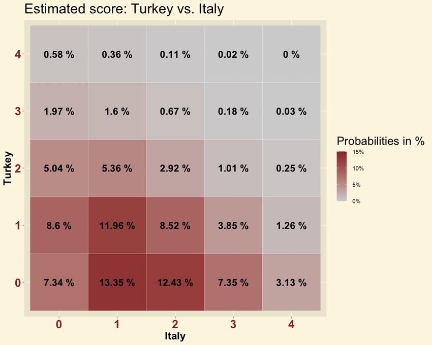
Since the basic element of our simulation is the simulation of single matches, we visualise
how to quantify the results of single matches. Group A starts with the match between
Turkey and Italy in Rome. According to our model we have the probabilities presented in
Figure 1 for the result of this match: the most probable scores are a 1 : 0 or 2 : 0 victory
of Italy or a 1 : 1 draw.
Figure 1. Probabilities for the score of the match Turkey vs. Italy (group
A) in Rome.
4.1. Group Forecast. In the following tables 5-10 we present the probabilities obtained
from our simulation for the group stage, where we give the probabilities of winning the
group, becoming runner-up, getting qualified for the round of last 16 as one of the best
ranked group third (Third Q), or to be eliminated in the group stage. In Group F, the
toughest group of all with world champion France, European champion Portugal and Ger-
many, a head-to-head fight between these countries is expected for the first and second
place.UEFA EURO 2020 FORECAST VIA NESTED ZIGP REGRESSION 11
Team GroupFirst GroupSecond Third Q Prelim.Round
Italy 39.8 % 28.3 % 15.8 % 16.10 %
Switzerland 24.1 % 26.9 % 19.6 % 29.40 %
Turkey 23.7 % 25.5 % 19.1 % 31.80 %
Wales 12.5 % 19.3 % 18.7 % 49.60 %
Table 5. Probabilities for Group A
Team GroupFirst GroupSecond Third Q Prelim.Round
Belgium 72.8 % 21.2 % 4.6 % 1.30 %
Denmark 19.9 % 42.9 % 17.9 % 19.30 %
Finland 3.8 % 14.4 % 15.4 % 66.40 %
Russia 3.5 % 21.4 % 18.4 % 56.70 %
Table 6. Probabilities for Group B
Team GroupFirst GroupSecond Third Q Prelim.Round
Netherlands 57.8 % 27.5 % 9.7 % 5.00 %
Ukraine 27.6 % 35.4 % 17.4 % 19.60 %
Austria 10.6 % 24.9 % 24.9 % 39.70 %
North Macedonia 4.1 % 12.3 % 14.5 % 69.20 %
Table 7. Probabilities for Group C
Team GroupFirst GroupSecond Third Q Prelim.Round
England 54.5 % 27.5 % 11.1 % 6.90 %
Croatia 26.5 % 32.9 % 17.6 % 22.90 %
Czechia 12.4 % 23.2 % 22.3 % 42.10 %
Scotland 6.6 % 16.4 % 17.7 % 59.20 %
Table 8. Probabilities for Group D
Team GroupFirst GroupSecond Third Q Prelim.Round
Spain 71.9 % 19.8 % 5.9 % 2.40 %
Sweden 12.6 % 34 % 20.6 % 32.80 %
Poland 12 % 31.6 % 21.6 % 34.90 %
Slovakia 3.6 % 14.6 % 14.1 % 67.60 %
Table 9. Probabilities for Group E12 LORENZ A. GILCH
Team GroupFirst GroupSecond Third Q Prelim.Round
France 37.7 % 30.4 % 17.9 % 14.00 %
Germany 32.4 % 30.3 % 19.9 % 17.40 %
Portugal 26.4 % 29.9 % 23 % 20.60 %
Hungary 3.5 % 9.5 % 11.8 % 75.10 %
Table 10. Probabilities for Group F
4.2. Playoff Round Forecast. Our simulations yield the following probabilities for each
team to win the tournament or to reach certain stages of the tournament. The result
is presented in Table 11. The ZIGP regression model favors Belgium, followed by the
current world champions from France and Spain. The remaining teams have significantly
less chances to win the UEFA EURO 2020.
Team Champion Final Semifinal Quarterfinal Last16
Belgium 18.4 % 29.1 % 47.7 % 68.7 % 98.5 %
France 15.4 % 24.9 % 38.8 % 58.4 % 85.9 %
Spain 13 % 22.5 % 38.9 % 68.1 % 97.7 %
England 7.8 % 14.8 % 26.8 % 50.5 % 93 %
Portugal 7.7 % 15.5 % 28.6 % 47.7 % 79.5 %
Netherlands 7.1 % 14.7 % 28.9 % 54.4 % 95 %
Germany 6.1 % 13.6 % 27.4 % 47.3 % 82.6 %
Italy 4.8 % 10.7 % 22.7 % 47.7 % 83.9 %
Turkey 3.7 % 8% 17.1 % 35.2 % 68.2 %
Denmark 3.5 % 9.2 % 20.8 % 40.7 % 79.7 %
Croatia 3.4 % 8.3 % 17.7 % 38.1 % 76.9 %
Switzerland 3.2 % 7.9 % 17.9 % 37.6 % 70.6 %
Ukraine 1.8 % 5.1 % 13.2 % 34.4 % 80.4 %
Poland 1.2 % 3.9 % 10.9 % 29.6 % 66.6 %
Sweden 1.1 % 3.9 % 10.8 % 30.9 % 68.6 %
Wales 0.6 % 2.2 % 7.2 % 19.7 % 50.6 %
Czechia 0.4 % 1.7 % 5.9 % 19.6 % 57.9 %
Russia 0.2 % 1% 4.1 % 12.9 % 41.5 %
Finland 0.1 % 0.7 % 2.6 % 9% 32.3 %
Austria 0.1 % 0.6 % 3.3 % 15 % 60.3 %
Slovakia 0.1 % 0.7 % 2.7 % 10.1 % 34 %
Hungary 0.1 % 0.6 % 2.6 % 8.3 % 24.7 %
Scotland 0.1 % 0.5 % 2.3 % 10.6 % 40.7 %
North Macedonia 0 % 0.1 % 0.9 % 5.5 % 30.8 %
Table 11. UEFA EURO 2020 simulation results for the teams’ probabili-
ties to proceed to a certain stageReferences 13
5. Final remarks
As we have shown in Subsection 2.5 the proposed ZIGP model with weighted historical
data seems to improve the model which was applied in (Gilch, 2019) for CAF Africa Cup
of Nations 2019. For further discussion on adaptions and different models, we refer once
again to the discussion section in (Gilch and Müller, 2018) and (Gilch, 2019).
References
Consul, P. (1989). Generalized Poisson distributions: Properties and Applications. Statis-
tics, textbooks and monographs v. 99. New York, M. Dekker.
Elo, A. E. (1978). The rating of chessplayers, past and present. Arco Pub., New York.
Gásques, R. and Royuela, V. (2016). The determinants of international football success:
A panel data analysis of the elo rating*. Social Science Quarterly, 97(2):125–141.
Gilch, L. A. (2019). Prediction Model for the Africa Cup of Nations 2019 via Nested
Poisson Regression. African Journal of Applied Statistics, 6(1):599–615.
Gilch, L. A. and Müller, S. (2018). On Elo based prediction models for the FIFA Worldcup
2018. Technical Report, Number MIP-1801, Department of Informatics and Mathe-
matics, University of Passau, Germany.
Ley, C., de Wiele, T. V., and Eetvelde, H. V. (2019). Ranking soccer teams on basis of
their current strength: a comparison of maximum likelihood approaches. Statistical
Modelling, 19:55–77.
Stekeler, D. (2004). Verallgemeinerte Poissonregression und daraus abgeleitete zero-inflated
und zero-hurdle Regressionsmodelle. Master’s thesis, Technical University of Munich.
Lorenz A. Gilch: Universität Passau, Innstrasse 33, 94032 Passau, Germany
Email address: Lorenz.Gilch@uni-passau.de
URL: http://www.math.tugraz.at/∼gilch/You can also read