Author response to comments by anonymous referee#1
←
→
Page content transcription
If your browser does not render page correctly, please read the page content below
Author response to comments by anonymous referee#1

Major comments
“Why did you limit the comparison of your results with only four models? In sections 3 and 4,
the large-scale features of this model should be briefly compared with other models. Such
simple comparisons may be effective to demonstrate that the dynamic vegetation or idealized
closed gateways are unique points of this study compared to the other PlioMIP2 studies.”
We apologize if our formulation was ambiguous here. We wrote:
“The COSMOS is of comparably low spatial resolution and there is only one other PlioMIP2
climate model that employs a similarly low resolution in the atmosphere. The COSMOS is also an
older model in the PlioMIP2 model ensemble, in particular in comparison to four PlioMIP2 models
that were published since 2017. Hence, the model is not anymore state–of–the–art.”
Our aim in this paper is actually focused on presenting the simulations that we contribute to the
PlioMIP2 ensemble; our aim is not so much to compare results from our model to those derived
from other models. The model-intercomparison within PlioMIP2 is the focus of the ensuing model-
model-intercomparison phase. There is already one such publication present that studies the model-
model intercomparison of large-scale features of Mid-Pliocene climate (Haywood et al., 2020).
In the text passage, that anonymous referee #1 points to, we actually just wanted to clarify that
some characteristics (not results) of our model are different to those from other models. We argued
based on an already available overview of characteristics of the contributing models (Table 1 of
Haywood et al., 2020). Our aim was not to refer to detailed results from individual models.
Yet, we fully acknowledge that anonymous reviewer #1 has a valid point in that we could present a
– very brief – summary of differences in large scale characteristics of mid-Pliocene climate
produced with our model in comparison to other studies. Since an extensive and very detailed
model-model-intercomparison has already been presented by Haywood et al. (2020), we will base
our comparison on the overview on PlioMIP2 model results presented by them.
We feel that a comparison of our results to those from other modelling groups has, in the context of
this model description paper, rather the characteristic of a discussion (more precisely, a discussion
of the comparison of our results to those by other modelling groups). We believe such text is not a
genuine part of the results section. Hence, we add the model comparison as an additional subsection
to section 4 “Discussion”. We will place this new subsection right at the start of section 4, so that
subsection 4.1, “The added value of COSMOS Mid-Pliocene simulations in PlioMIP2”, will
become subsection 4.2 in a revised manuscript.
The additional subsection will be named “4.1 Comparison of selected Mid-Pliocene large scale
climate patterns to the PlioMIP2 model ensemble”. The text will be incorporated in a revised
version of the manuscript.
Unfortunately, we will not be able to produce a model-intercomparison that aims at quantification
of the importance of dynamic vs. prescribed vegetation, and at modern vs. Pliocene gateways,
which the reviewer aims at. There are no other model simulations that employ dynamic vegetation
(see Table 1 by Haywood et al., 2020), and our model seems to be the only one for which a
dedicated PlioMIP2 mid-Pliocene simulation with modern gateways is available. Hence, we lack
the data from other models on which we could base a robust multi-model comparison “dynamic vs.
fixed vegetation” and “modern vs. reconstructed gateways”.

                                                 1
“It is much better to add figure showing evolutions of SAT (and AMOC or deep ocean
temperature, for example) during the model integrations, especially for e280, eoi400 and
eoi400_GW runs, similar to what you showed in your previous paper (Figure 6 of 2012 GMD
paper). It would be OK to include it into the supplement if there would be nothing particular
to be noted in the main text.”
We thank the reviewer for the proposal to better highlight the state of equilibrium of our
simulations, beyond what has already been done based on Table 2 (column “TOA imbalance”) of
our manuscript. We already have prepared an illustration that shows the evolution of global average
potential temperature in the ocean over the spinup- and analysis-periods of the various PlioMIP2
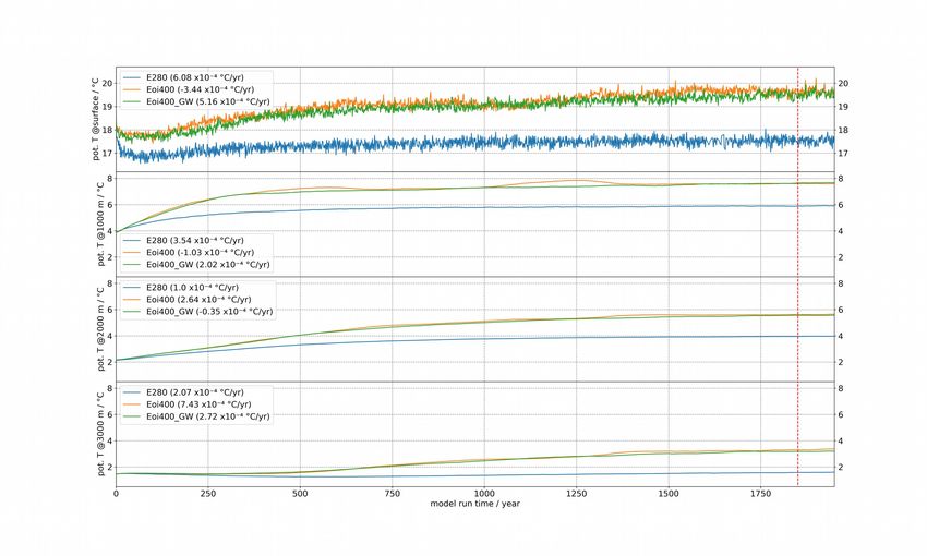
simulations with COSMOS. As suggested by reviewer #1, we propose to present an analysis of the
time evolution of ocean temperature in simulations E280, Eoi400, and Eoi400_GW at the surface,
and at three different ocean depth layers (1000 m, 2000 m, and 3000 m) in a supplement to the
manuscript. Yet, we propose to show SST, that is closely coupled to SAT outside sea ice regions,
instead of SAT, towards a better comparability of surface temperature and subsurface ocean
temperature. This supplementary figure is presented at the end of this comment. In the main text we
refer to this supplementary analysis in the following manner by means of an extension of the text at
page 13, line 15 (new text in red):
“The simulated Mid-Pliocene climate state Eoi400 is over the analysis period slightly less
equilibrated (by 0.16 W m²) than the reference climate state E280, as evidenced by top of the
atmosphere (TOA) radiative imbalance. The generally high TOA radiative imbalance across the
simulation ensemble (1.7–2.0 W m²) is comparable to imbalances in the model that are present in
the framework of PlioMIP1 (Stepanek and Lohmann, 2012). Radiative imbalance is related to the
slow response of the ocean to changes in carbon dioxide forcing as shown before (Li et al., 2013).
In our case, a combination of changes in carbon dioxide and geographic boundary conditions causes
a slow equilibration process that is not fully finished at the end of the model spinup (Fig. S1 in the
supplement to this article). In particular, simulation Eoi400 still exhibits a temperature trend of
about 7·10 ⁴ °C yr ¹ at 3000 m depth over the analysis period. On the other hand, the ocean surface,
on which PlioMIP2 analyses focus heavily, is in simulation Eoi400 in quasi-equilibrium. During the
analysis period, the simulation is subject to an ocean surface temperature trend that is actually
below the respective trend in the PI control state E280. Furthermore, the ocean surface slightly
cools in the analysed portion of Mid-Pliocene core simulation Eoi400. This suggests that the
diagnosed surface temperature trend is, from the view point of the ocean surface, largely
overprinted by internal variability. Similarity of TOA imbalance and small residual ocean surface
temperature trends across the PlioMIP2 COSMOS simulation ensemble demonstrate, despite
incomplete model equilibration, expediency of simulation Eoi400 and other COSMOS PlioMIP2
simulations for the study of climate anomalies.”
“Page 22, line 14: “a northward shift” Does this also mean a northward shift of vegetation in
the Southern Hemisphere? Or a poleward shift? If a northward shift is also found over the
Southern Hemisphere, it indicates a equatorward shift, contrasting to the NH. What are the
factors?”
Although the COSMOS simulate vegetation dynamics across the entire land surface of both the
Northern and Southern Hemisphere (with the exception of regions covered by ice sheets), our focus
on analysis is largely on vegetation shifts of the Northern Hemisphere. Polar amplification of global
climate anomalies is much larger in the Northern Hemisphere as evidenced in many other
publications for both future and Cenozoic climate, and this is also evident in our simulation
ensemble. At the text location, to which the reviewer points, we actually specifically talk about
northward shifts in the Northern Hemisphere, and we clarify the text in a revised manuscript
accordingly.
2Regarding the question “What are the factors?” we assume that the reviewer asks us to link shifts in
vegetation cover to changes in the simulated climate variables, foremost temperature and
preciptation. We have analysed the correlation between simulated vegetation cover and monthly
mean climate variables independently of this manuscript. This research has produced a complex
picture on correlations between climate and vegetation. This is understandable as the analysis has to
go beyond simulated climate and must also consider changes in the prescribed soil cover and the
various PFT’s tolerance to extremes in temperature and rain. To present such an analysis we would
have to include additional data that is beyond the monthly averages of temperature and precipitation
presented in our publication. Currently, we are analysing climate extremes in the Pliocene. Studying
the response of vegetation will likely be a part of this. Yet, we fear that additional information, that
needs to be conveyed towards a proper analysis of the factors, is well beyond the scope of this
modelling paper and must be left for a future publication.
Specific comments
Page 13, line 20: lower elevation and the absence of ice sheets
The suggested change has been implemented into a revised manuscript.
Page 14, line 9-16: The discussion here is closely related to variation in ITCZ related to
interhemispheric asymmetry in energy balance. It is better to refer any previous studies here, for
example doi: 10.1175/2007JCLI2146.1.
We thank the reviewer for pointing out that reporting our results could be done in a less descriptive
way, paying more attention to the mechanisms behind the changes in low latitude rain patterns. We
refer now to previous literature, pointing out the connection between asymmetry of
interhemispheric energy balance and related shifts of precipitation patterns in low latitudes.
Consequently, we have added the following text at the end of line 16:
“Pronounced changes in low-latitude precipitation, Mid-Pliocene vs. PI, are related to the
asymmetric warming between hemispheres. It has been shown by various authors that the ITCZ
shifts towards the warmer hemisphere via links between tropical and extratropical climate (Haug et
al., 2001; Broccoli et al., 2006; Kang et al., 2008; Deplazes et al., 2013; Schneider et al., 2014). The
warmer hemisphere is in our Mid-Pliocene simulations the Northern Hemisphere, that warms more
widespread than the Southern Hemisphere and across all seasons (Fig. 3).”
Page 14, line 33: model. Raomo et al.
We agree with the reviewer that the sentence was far too long to easily grasp it’s meaning. We have
split the text accordingly as follows (changes in red):
“In contrast, we find that the maximum stream function of the Atlantic Meridional Overturning
Circulation (AMOC) is increased in simulation Eoi400 (Table 4) with respect to simulation E280.
Hence, our model confirms Raymo et al. (1996) and Dowsett et al. (2009) in that Mid-Pliocene
thermohaline circulation was higher than today.”
Page 24, line 6: to to
Erroneous repeating of the word “to” has been fixed.
3References
Broccoli, A. J., Dahl, K. A., and Stouffer, R. J.: Response of the ITCZ to Northern Hemisphere
cooling, Geophys. Res. Lett., 33, L01702, doi:10.1029/2005GL024546, 2006.
Deplazes, G., Lückge, A., Peterson, L., Timmermann, A., Hamann, Y., Hughen, K. A., Röhl, U.,
Laj, C., Cane, M. A., Sigman, D. M., and Haug, G. H.: Links between tropical rainfall and
North Atlantic climate during the last glacial period, Nature Geosci., 6, 213–217, https://doi.org/
10.1038/ngeo1712, 2013.
Dowsett, H. J., Robinson, M. M., and Foley, K. M.: Pliocene three-dimensional global ocean
temperature reconstruction, Clim. Past, 5, 769--783, https://doi.org/10.5194/cp-5-769-2009,
2009.
Haug, G. H., Hughen, K. A., Sigman, D. M., Peterson, L. C., and Röhl, U.: Southward Migration of
the Intertropical Convergence Zone Through the Holocene, Science, 293, 1304–1308,
https://doi.org/10.1126/science.1059725, 2001.
Haywood, A. M., Tindall, J. C., Dowsett, H. J., Dolan, A. M., Foley, K. M., Hunter, S. J., Hill, D. J.,
Chan, W.-L., Abe-Ouchi, A., Stepanek, C., Lohmann, G., Chandan, D., Peltier, W. R., Tan, N.,
Contoux, C., Ramstein, G., Li, X., Zhang, Z., Guo, C., Nisancioglu, K. H., Zhang, Q., Li, Q.,
Kamae, Y., Chandler, M. A., Sohl, L. E., Otto-Bliesner, B. L., Feng, R., Brady, E. C., von der
Heydt, A. S., Baatsen, M. L. J., and Lunt, D. J.: A return to large-scale features of Pliocene
climate: the Pliocene Model Intercomparison Project Phase 2, Clim. Past Discuss.,
https://doi.org/10.5194/cp-2019-145, in review, 2020.
Kang, S. M., Held, I. M., Frierson, D. M., and Zhao, M.: The Response of the ITCZ to Extratropical
Thermal Forcing: Idealized Slab-Ocean Experiments with a GCM, J. Climate, 21, 3521–3532,
https://doi.org/10.1175/2007JCLI2146.1, 2008.
Li, C., von Storch, J., and Marotzke, J.: Deep-ocean heat uptake and equilibrium climate response,
Clim. Dyn., 40, 1071--1086, https://doi.org/10.1007/s00382-012-1350-z, 2013.
Raymo, M. E., Grant, B., Horowitz, M., and Rau, G. H.: Mid-Pliocene warmth: stronger greenhouse
and stronger conveyor, Mar. Micropaleontol., 27, 313--326, https://doi.org/10.1016/0377-
8398(95)00048-8, 1996.
Schneider, T., Bischoff, T., and Haug, G.: Migrations and dynamics of the intertropical convergence
zone, Nature, 513, 45–53, https://doi.org/10.1038/nature13636, 2014.
Stepanek, C. and Lohmann, G.: Modelling mid-Pliocene climate with COSMOS, Geosci. Model
Dev., 5, 1221--1243, https://doi.org/10.5194/gmd-5-1221-2012, 2012.
4Supplement to cp-2020-10
Figure S1: Time evolution of potential seawater temperature at various ocean depths between
surface and 3000 m as a diagnostic for model equilibration. Shown is the evolution of temperature
over the runtime of PlioMIP2 COSMOS core simulations Eoi400 and E280 and of the sensitivity
study with Mid-Pliocene geography but modern states of Bering Strait, Hudson Bay, and Canadian
Arctic Archipelago, Eoi400_GW. Vertical red bars denote the start of the PlioMIP2 analysis period
that ends at model year 1949 at the end of the time period shown in the illustration. Temperature
trends during the analysis period are given in brackets in the legend after the respective simulation
name. These indicate that simulations are in a quasi-equilibrium over the PlioMIP2 analysis period.
Note the difference in scale between ocean surface and ocean subsurface temperatures.
5You can also read