Updating the United States Government's Social Cost of Carbon - Tamma Carleton and Michael Greenstone

WORKING PAPER · NO. 2021-04

Updating the United States Government’s
Social Cost of Carbon
Tamma Carleton and Michael Greenstone
JANUARY 2021

 5757 S. University Ave.
 An Affiliated Center of
 Chicago, IL 60637
 Main: 773.702.5599
 bfi.uchicago.edu

Updating the United States Government’s Social Cost of Carbon

 Tamma Carleton
 Bren School of Environmental Science & Management
 University of California, Santa Barbara

 Michael Greenstone
 Department of Economics
 University of Chicago
 NBER

 Abstract

 This paper outlines a two-step process to return the United States government’s
 Social Cost of Carbon (SCC) to the frontier of economics and climate science.
 The first step is to implement the original 2009-2010 Inter-agency Working
 Group (IWG) framework using a discount rate of 2%. This can be done
 immediately and will result in an SCC for 2020 of $125. The second step is to
 reconvene a new IWG tasked with comprehensively updating the SCC over the
 course of several months that would involve the integration of multiple recent
 advances in economics and science. We detail these advances here and provide
 recommendations on their integration into a new SCC estimation framework.

We thank Jared Stolove for exceptional research assistance and Trevor Houser, Amir Jina, Robert Kopp,
Ishan Nath, and Cass Sunstein for valuable critiques and suggestions. This working paper will also appear
in a forthcoming book of energy and environmental policy proposals to be published by the Energy Policy
Institute at the University of Chicago (EPIC). Contact information: tcarleton@ucsb.edu and
mgreenst@uchicago.edu.

I. Heart of the Problem

All over the world, climate policies have the potential to provide large benefits by
reducing the harms that result from carbon dioxide (CO2) emissions. However, these
policies can be costly, with some more expensive than others. The value of reducing
such emissions is not $0, and it is not infinite. Some imaginable fuel economy standards,
for example, would be very stringent, while others would be very lenient. What level of
stringency is optimal, if a central goal of those standards is to reduce carbon dioxide
emissions? To confront the challenge of climate change effectively, the public is best
served by policies that have benefits in excess of costs, and that maximize net benefits.

A key tool in identifying such policies is the social cost of carbon (SCC), which
represents the monetized damages associated with a one metric ton increase in CO2
emissions. In principle, the SCC illustrates the dollar value all of the future damages
associated with the change in climate due to the release of an additional ton of CO2,
including (but not limited to), mortality and other health effects from excess heat and
natural disasters, depressed agricultural production, reductions in labor productivity,
disruption of energy systems, increased risk of violent conflict, property damage from
hurricanes and floods, and mass migration out of affected regions. The SCC therefore
reflects how much society should be willing to pay to reduce carbon dioxide emissions
by a ton.

With this information, policymakers can easily conduct cost-benefit analysis of
regulations that reduce CO2 emissions. The costs to the economy of lowering emissions
(e.g., imposing fuel economy standards on car manufacturers) are naturally calculated in
dollars. And with the SCC, the benefits of CO2 emissions reductions are converted into
dollars. The result is an apples-to-apples comparison of an individual regulation’s
benefits and costs, both measured in dollars.

From the standpoint of law and practice, this conversion is extraordinarily helpful. In
the United States, some legislation formally requires agencies to conduct cost-benefit
analysis, and prevailing Executive Orders, supported by both Republican and
Democratic presidents, require such an analysis for all major regulations, including those
designed to reduce carbon emissions. Though the use of cost-benefit analysis is not

 2

without controversy, there is a strong argument in favor of conducting such an analysis,
and giving serious consideration to it, if the goal is to ensure that regulations best
promote the American people’s interests.1

Following the Supreme Court’s decision in U.S. EPA vs. Massachusetts (2007), the U.S.
government has been required to issue at least some regulations to reduce greenhouse
gas emissions, but it lacked a consistent SCC with which to inform its judgments. In
2009, therefore, the Obama administration issued a temporary SCC and formed an
Inter-agency Working Group (IWG) that was tasked with developing a robust SCC,
based on the best available science and economics. The work was completed in 2010 and
then successively updated, which ultimately produced a value of $52 per ton of CO2 in
2020.2 The same methods were used to develop a social cost of methane, another potent
greenhouse gas, in 2016.3 Following a request from the Obama administration, the
National Academies of Sciences, Engineering, and Medicine (NAS) released a report on
how to bring the SCC closer to the frontier of climate science and economics in January
2017.

Not long after that report’s release, the Trump administration disbanded the IWG and
reduced the SCC to between $1 and $7 (see left panel of Figure 1), making changes in
assumptions that did not follow the NAS recommendations and that were difficult to
justify based on science and economics.4 In the past four years, the controversial and
substantially lower SCC estimates used by the Trump administration have helped to
pave the way for the rollback of environmental regulations. For example, as illustrated
in Figure 2, the Trump administration’s 2017 reconsideration and substantial weakening
of Obama-era fuel economy standards was merited, on cost-benefit grounds, with its
lower SCC, but would not have been so justified with the IWG SCC.

1 Livermore and Revesz, Reviving Rationality.
2 Interagency Working Group, “Technical Support Document” (2013).
3 Interagency Working Group, “Technical Support Document” (2016).
4 Greenstone, Congressional Testimony.

 3

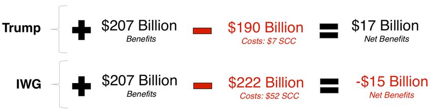
Figure 1: Current U.S. Social Cost of Carbon (SCC) is behind frontier science. This figure compares
current and past U.S. federal SCCs to those produced by recent scientific and economic research. The full
all-sector SCCs shown on the left are U.S. federal SCCs used under the Obama administration (grey) and
the Trump administration (brown). Sector-specific “partial” SCCs on the right come from the Interagency
Working Group (IWG) 2013 implementation of the FUND model (grey) and recent scientific literature
(blue). Sources: Rode et al. (2020b), Carleton et al. (2020), Moore et al. (2017), and Anthoff and Tol
(2014), as decomposed by Diaz (2014). All estimates indicate the willingness-to-pay to avoid an increase
in emissions in the year 2020, are shown in 2020 USD, rely on an approximate “business-as-usual”
emissions scenario (e.g., RCP 8.5), and use a 3 percent discount rate.

Since its release in 2010, the SCC has played a central role in climate policy both
domestically and internationally. For example, as of 2017 the federal government had
used the SCC to assess the value of over eighty regulations with a combined $1 trillion
in estimated gross benefits.5 At least eleven state governments have begun using an SCC
to guide policy, most notably in Illinois and New York, where governments use the SCC
to value “zero-emissions credits” paid to producers of clean energy.6 Meanwhile, several
other countries, including Canada, France, Germany, Mexico, Norway, and the United

5 Nordhaus, “Revisiting the Social Cost of Carbon.”
6 Institute for Policy Integrity, “The Cost of Carbon Pollution.”

 4

Kingdom, have referred to the experience of the United States to implement their own
SCC estimates, with some adopting estimates wholesale from the IWG.7

Figure 2: Current U.S. SCC used to justify rollbacks of fuel-economy standards. Figure displays an
example regulatory cost-benefit analysis (CBA) using two different SCCs. The values shown are the costs
and benefits of a 2017 Environmental Protection Agency (EPA) and National Highway Traffic and Safety
Administration (NHTSA) rollback of fuel economy standards for 2021-2026 model-year vehicles. The top
row displays the benefits and costs of the rollback using the 2017 Trump administration 3 percent
discount rate SCC, taken directly from Table I-I and Table VII-286 of EPA and NHTSA (2017). The
bottom row uses the same benefit estimate, but calculates the costs using the 2013 IWG 3 percent
discount rate SCC (i.e., the Obama administration SCC), leaving all other assumptions the same across
rows (IWG, 2013). Cost estimates incorporate damages from carbon emissions and other factors, such as
the monetary cost of fuel. Costs from sources other than carbon emissions account for $178 billion of costs
in both rows. Both costs and benefits are converted from 2018 to 2020 dollars using the BEA CPI
inflation calculator.

In many respects, the SCC is the “straw that stirs the drink” for most domestic climate
policies, determining in some cases whether or not regulatory action can proceed.8 But
the national SCC can also influence the direction of international climate negotiations:
experience demonstrates that meaningful U.S. action can leverage large reductions in
emissions from other countries that reduce the climate damages that Americans must
contend with.9

Rapid scientific and economic advances in the last decade mean that there is now an
urgent need to update the SCC. The Obama-era SCC relied on the science and data

7 U.S. GAO, “Social Cost of Carbon”
8 Sunstein, “Watch for Biden Decision on Unsung Climate Metric.”
9 Houser, “Calculating the Climate Reciprocity Ratio.”

 5

available at the time, often making simplifying assumptions that are now understood to
be invalid or unnecessary. Recognizing the likely advance of understanding, the IWG
explicitly called for “update[s] over time to reflect increasing knowledge of the science
and economics of climate impacts.”10 Despite some incremental changes, however, a
wholesale update was never conducted. The consequence is that neither the Trump nor
Obama SCC incorporates the explosion of data and research since 2010 that has
dramatically expanded knowledge of the climate, economy, and the relationship between
the two. A defining feature of the best new research is that it relies on large-scale data
sets, rather than assumptions that are often unverifiable.

A number of these new, empirically grounded studies indicate that the underpinnings of
the current SCC are no longer valid in terms of, for example, their projected impacts on
mortality rates, energy demand, and agricultural productivity.11 The right panel of
Figure 1 shows three of the sector-specific component or “partial” SCC estimates
developed in recent years (blue), as they compare to the same components of the federal
SCC developed in 2013 (grey). New estimates for two of three recently studied SCC
sectors (mortality and agriculture) indicate substantially larger damages from CO2,
suggesting that the SCC, as settled in 2013, is too low.

Besides advancing understanding about the overall impacts of climate change, these
data-driven updates to the SCC have uncovered large differences in the impacts of
climate change both within and across countries that were invisible with previous
approaches. The key finding is that climate change is projected to disproportionately
harm today’s poorest populations, exacerbating concerns about environmental justice.12
These distributional findings are only visible with the detailed data that characterize the
new wave of research. As just one example, even within a wealthy country like the
United States, climate change is projected to cause economic damages in the poorest 5
percent of counties that are approximately nine times larger on average by the end of
the century than in those in the richest 5 percent.13 Put plainly, this new research

10 Interagency Working Group, “Technical Support Document” (2010).
11 Carleton et al., “Valuing the Global Mortality”; Rode et al., “Estimating a Social Cost of Carbon”; Diaz
& Moore, “Quantifying the Economic Risks”; Moore et al., “New Science of Climate Change Impacts”.
12 See, for instance, Hsiang et al., Estimating Economic Damage from Climate Change in the United

States.”
13 Id

 6

makes it possible to assess who is most affected by climate policies—insight that is out
of reach under the current SCC framework.

Revising the U.S. SCC based on a new and more durable foundation would return the
SCC to the frontier of understanding about the risks from climate change and lead to
better policy that protects Americans against unnecessary climate risks. Moreover, such
an update would undoubtedly influence policy abroad, which directly affects the well-
being of Americans, since the climate is equally affected by emissions from Chicago, as
those from Beijing, Mumbai, Paris, and Riyadh.

This paper outlines a two-step approach to updating the U.S. SCC that returns it to the
frontier of knowledge. The Biden administration can initiate the first step immediately
and simply involves implementing the IWG’s approach again with a discount rate of no
higher than 2 percent, which reflects profound changes in international capital markets
that make the current values difficult to justify. At a discount rate of 2% the SCC in
2020 is $125.14

The second step is for the Biden administration to launch a reconstituted IWG and task
it with a comprehensive updating of the SCC. There are seven key “ingredients” that
should go into such a process and the next section identifies each of them, explains what
was done in the past, describes how understanding has advanced since 2009-2010, and
makes a specific recommendation. The paper’s final section details multiple pathways
towards combining these ingredients to produce an updated SCC. Importantly, none of
these pathways can be implemented immediately; a reconstituted IWG’s work could
take several months.

II. The Seven Key Ingredients for a Revised SCC

Calculating the SCC requires a model that accounts for the future growth of the
economy, the relationship between emissions and climate change, the effect of climate
change on the economy, and a number of other factors. Such models are referred to as
Integrated Assessment Models (IAMs), since they combine scientific and economic

14New York State Department of Environmental Conservation, “Establishing a Value of Carbon”; New
York State Energy Research and Development and Resources for the Future, “Estimating the Value of
Carbon: Two Approaches.”

 7

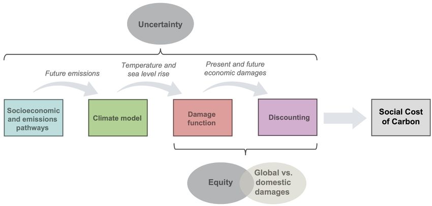
models to evaluate the impacts of carbon emissions. The Obama-era IWG estimated the
SCC using three existing IAMs—DICE, FUND, and PAGE—which were developed in
the 1990s and have been widely used in the economic and scientific literature.15

There are seven “ingredients” necessary to construct the SCC. The first four are often
referred to as “modules” (see Figure 3):

 1. A socioeconomic and emissions trajectory, which predicts how the global
 economy and CO2 emissions will grow in the future;
 2. A climate module, which measures the effect of emissions on the climate;
 3. A damages module, which translates changes in climate to economic
 damages; and
 4. A discounting module, which calculates the present value of future
 damages.

In addition, there are three cross-cutting modeling decisions that affect the entire
process:

 1. Whether to include global or instead only domestic climate damages;
 2. How to value uncertainty; and
 3. How to treat equity.

15Nordhaus, “Economic Aspects of Global Warming”; Anthoff and Tol, “The Income Elasticity of the
Impact of Climate Change”; Hope, “The PAGE09 Integrated Assessment Model.”

 8

Figure 3: Seven ingredients for calculating the Social Cost of Carbon. This figure displays the four
“modules” that compose the SCC (colored boxes), and the three key modeling decisions (grey ovals) that
together form the seven “ingredients” necessary to compute an SCC.

Updating the SCC so that it is built on a foundation of frontier science and economics
would require a newly constituted IWG to make decisions regarding each of these seven
ingredients. However, the IWG need not start from scratch; some required updates are
already clear. Due to significant advances in climate modeling and in climate impact
analysis, as well as profound changes in global capital markets, it is essential to update
the climate and damage modules and to change the rate of discounting. It is additionally
essential to update the Trump administration’s U.S. SCC to reflect global, as opposed to
domestic only, damages, based on an overwhelming consensus amongst scientific and
economic experts. Failing to account for these advances would leave any new SCC open
to well-founded scientific criticism. It could also leave a new SCC vulnerable to legal
invalidation; courts review agency decisions to ensure that they are not “arbitrary or
capricious,” and if a new SCC were not based on scientific advances it could be
challenged on exactly that ground. There are also valuable opportunities to update the
other three ingredients, but to varying degrees the scientific and/or policy case for doing
so is less urgent.

This paper can be thought of as a “recipe,” outlining ways to bring the U.S.
government’s SCC back up to the scientific frontier. This section briefly explains each of

 9

the seven key ingredients, describes how they were handled by the IWG in 2010, and
makes recommendations to update each.

 A. Essential Updates to the SCC

Ingredient 1: Climate Module

Background: The development of an SCC requires a climate model that converts carbon
emissions into changes in the global climate. Specifically, these models must characterize
the relationship between emissions and atmospheric CO2 concentrations and the
relationship between atmospheric CO2 and changes in the climate, including both
warming and sea level rise. All three IAMs used by the IWG included highly simplified
climate models. A core input into each of these models was the Equilibrium Climate
Sensitivity (ECS), which determines the total global warming realized from a doubling
of atmospheric carbon concentrations. The ECS has a substantial impact on the SCC
but its true value is not known with scientific certainty.

2010 IWG Approach: The IWG relied on the climate models within each IAM. However,
to ensure that the ECS values used reflected the best available science at the time, the
IWG harmonized the ECS across all models by using a probability distribution that
reflected the likelihood of different possible climate outcomes at the end of the century
according to the Intergovernmental Panel on Climate Change’s (IPCC) Fourth
Assessment Report. This was the only component of each IAM’s climate model that the
IWG calibrated to match scientific evidence.

Progress: Recent evidence makes clear that the IAMs used to calculate the IWG SCC,
even with a harmonized ECS, are outdated, as they do not reflect a substantial body of
new research quantifying multiple links in the causal chain from emissions to
temperature change.16 In particular, DICE, FUND, and PAGE substantially
underestimate the speed of temperature increase, relative to climate models that satisfy
the NAS criteria for meeting scientific standards (Figure 4).17 For example, higher
atmospheric CO2 concentrations cause the oceans to warm and acidify, which makes

16 Dietz et al., “Are Economists Getting Climate Dynamics Right”; Mattauch et al., “Steering the Climate
System”; NAS, “Valuing Climate Damages.”
17 NAS, “Valuing Climate Damages,” Recommendation 4-1

 10

them less effective at removing CO2 from the atmosphere. The consequence is a positive
feedback loop that accelerates warming.18 However, this dynamic is missing from both
the DICE and PAGE climate modules.

The fact that existing IAMs do not reflect the well-developed climate science literature
substantially influences the magnitude of the SCC.19 Importantly, the delayed projection
of warming in the IAMs’ climate models means that resulting estimates of the SCC are
likely to be too low. The delay pushes warming further into the future, which is
discounted more heavily, as shown in the bottom panel of Figure 4.

Figure 4: Current Integrated Assessment Models do not reflect well-developed climate science. Dynamic
temperature response to a 100GtC impulse of CO2 from the CMIP5 climate model ensemble (red solid
line, labeled “best available climate science”) versus the three IAMs used to compute the U.S.
government’s SCC (DICE, FUND, and PAGE). The lower panel shows the present discounted value of
$1, discounted using a 2 percent discount rate. Source for top panel: Dietz et al., 2020.

Recommendation: It is vital that an updated SCC relies on a climate model that
accurately reflects the climate system’s functioning. Because any SCC calculation
requires fully capturing the uncertainty surrounding the impact of CO2 on temperature

18 Dietz et al., “Are Economists Getting Climate Dynamics Right.”
19 Id

 11

and other climate variables, however, it would be computationally infeasible to replace
IAM climate models with state-of-the-art Earth system models that capture the physics,
chemistry, and biology of the atmosphere, oceans and land at high spatial resolution.
Therefore, a simple Earth system model that can conduct uncertainty analysis while also
matching predictions from these more complex models is necessary.

The first part of our20 climate model recommendation is that IWG use the simple Earth
system model FAIR to project changes in temperature.21 The FAIR model satisfies all
criteria set by the NAS for use in an SCC calculation.22 Importantly, this model
generates projections of future warming that are consistent with comprehensive, state-
of-the-art models and it can be used to accurately characterize current best
understanding of the uncertainty regarding the impact that an additional ton of CO2
has on global mean surface temperature (GMST). Finally, FAIR is easily implemented
and transparently documented,23 and is already being used in updates of the SCC.24

A key limitation of FAIR and other simple climate models is that they do not represent
the change in global mean sea level rise (GMSL) due to a marginal change in emissions.
However, statistical methods can be used in combination with long historical records of
both temperature and sea level to build a semi-empirical model of the relationship
between GMSL and GMST.25 Such models are readily available26 and can enable the
inclusion of marginal damages due both to warming and to projected changes in sea
level. An important potential caveat is that available semi-empirical models of GMSL,
in addition to more complex bottom-up models, may underestimate future sea level rise
due to their inability to capture plausible future dynamics that are not observed in the
historical record (e.g., ice cliff collapse).

20 Throughout, “we” or “our” refers solely to the views of Carleton and Greenstone and not necessarily
those of EPIC, the University of Chicago, or the University of California, Santa Barbara.
21 Millar et al., “A Modified Impulse-Response Representation.”
22 NAS, “Valuing Climate Damages.”
23 FAIR’s source code can be accessed here: https://github.com/OMS- NetZero/FAIR/.
24 Dietz et al. “Are Economists Getting Climate Dynamics Right”; Carleton et al., “Valuing the Global

Mortality Consequences”; Rode et al., “Labor Supply in a Warmer World”; Rode et al., “Estimating a
Social Cost of Carbon for Global Energy Consumption.”
25 NAS, “Valuing Climate Damages.”
26 See, for example, Kopp et al., “Temperature-Driven Global Sea-Level Variability.”

 12

The second part of our climate model recommendation is that the IWG use semi-
empirical models to project changes in sea level based on changes in global mean surface
temperature from FAIR.

Finally, a strength of simple climate models like FAIR is that they can project GMST,
accounting for climatological uncertainty, both with and without a marginal increase in
emissions, which is necessary to compute the social cost of one additional ton of CO2.
However, they are not able to provide local climate projections at, for example, the
county level. This introduces a challenge, as socioeconomic trajectories are available
nationally and, as discussed below, recovering a valid damage function requires that
climate impacts be estimated locally. It is possible, however, to use high spatial detail in
socioeconomic and climatic conditions to estimate damages that are then calibrated to
GMST (and GMSL, for sectors where sea level rise is an important driver of climate
change impacts) in a second stage.27

Therefore, the third part of our climate model recommendation is that the damage
function itself should relate total socioeconomic damages to changes in global mean
surface temperature (and global mean sea level rise where appropriate).

Ingredient 2: Damages Module

Background: A “damage function” translates changes in the physical climate (e.g.,
temperature and sea level rise) into monetized impacts on the economy. In some IAMs,
a single damage function is calibrated to represent all categories of climate impact (e.g.,
PAGE), while in others, separate damage functions are modeled for individual impact
categories (e.g., FUND). In DICE, a single damage function is used, but it is calibrated
based on individual sector-specific damage estimates.28

At least two problems have plagued the IAM damage functions. First, they are
primarily derived from ad-hoc assumptions and simplified relationships, not large-scale
empirical evidence. Further, the IAM damage functions have tended to treat the world
as nearly homogeneous, dividing the globe into at most sixteen regions. This aggregation

27 NAS, “Valuing Climate Damages”; Carleton et al., “Valuing the Global Mortality Consequences;” Rode
et al., “Labor Supply in a Warmer World;” Rode et al., “Estimating a Social Cost of Carbon for Global
Energy Consumption.”
28 Nordhaus, “The ‘DICE’ Model.”

 13

misses a great deal, especially because there are important nonlinearities in the
relationship between temperature and human well-being that are obscured by
substantial aggregation. For example, a given increase in temperature will have very
different impacts in Arizona than it will in northern Minnesota. For both of these
reasons, these damage functions have been heavily criticized in recent years.29

2010 IWG Approach: When the IWG developed the first SCC in 2010, existing IAM
damage functions were essentially the only feasible option. As a result, there were few if
any alternatives and the IWG kept the damage functions originally included in DICE,
FUND, and PAGE.

Progress: In the last dozen years, there have been great advances in computing power,
access to data from around the world, and econometric methods designed to quantify
climate change impacts. A result has been an explosion of empirical research that has
greatly deepened science’s understanding of the economic impacts of climate change.30
Relative to 2009, there is almost an embarrassment of riches, with, for example, at least
110 empirical studies on climate change’s economic impacts published between 2010 and
2016 alone.31

So how should one choose among all of these studies when developing an updated
damage function? To make full use of scientific advances, any modern damage function
must now meet three criteria:

 1. Empirically derived and plausibly causal: Damage functions should be derived
 from empirical estimates that reflect plausibly causal impacts of weather events
 on socioeconomic outcomes.

 Because the climate has remained stable throughout modern human history, it is
 difficult to isolate experimental variations in the long-run climate. However, a
 large and growing empirical literature leverages modern econometric methods to
 uncover causal impacts of short-run weather events on a host of socioeconomic

29 Pindyck, “Climate Change Policy: What Do the Models Tell Us?”
30 Carleton and Hsiang, “Social and Economic Impacts of Climate;” Dell et al., “What Do We Learn from
the Weather?”; Deschenes and Greenstone, “The Economic Impacts of Climate Change.”
31 Carleton and Hsiang, “Social and Economic Impacts of Climate.”

 14

outcomes, from agricultural output to mortality rates to energy use.32 When
 combined with empirical estimates of differences in populations’ responses to
 weather events (discussed in criterion three below), this literature provides a
 strong foundation for understanding the socioeconomic effects of weather, and its
 approach should be reflected in a new IWG’s damage function.

 The damage functions from FUND, DICE, and PAGE used by the IWG do not
 meet this criterion. They are only loosely calibrated to empirical evidence and/or
 rely on outdated estimates that fail to isolate the role of changes in the climate
 from economic variables such as income and institutions. For example, the
 majority of the studies used in FUND’s sector-specific damage functions were
 published prior to 2000, and all likely suffer from the influence of unobserved
 factors that are correlated with temperature. Similarly, early versions of DICE
 utilized a damage function that was only loosely tied to empirical literature (Diaz
 and Moore, 2017; Nordhaus, 2010), while the recent DICE update continues to
 rely on empirical papers that fail to identify plausibly causal effects (Nordhaus
 and Moffat, 2017).

 2. Capture local-level nonlinearities for the entire global population: Damage
 functions should be estimated with data that represent the entire global
 population (not just high-income, temperate regions). Further, damage functions
 should account for “nonlinear” effects of climate variables at a local level.

 Dramatic reductions in computing costs and increased data availability have
 enabled researchers to identify the effects of climate change on social and
 economic conditions at local scale across the globe. This body of work has
 uncovered that many socioeconomic outcomes display a strongly nonlinear
 relationship with climate variables—that is, the effects of climate change are not
 identical everywhere, but are instead sensitive to prior socioeconomic and
 climatic conditions.33 For example, both extreme cold and extreme heat increase
 mortality rates, while moderate temperatures have little impact.34 In addition,

32 Carleton and Hsiang, “Social and Economic Impacts of Climate;” Dell et al., “What Do We Learn from
the Weather?”
33 Carleton and Hsiang, “Social and Economic Impacts of Climate.”
34 Gasparinni et al., “Mortality Risk Attributable to High and Low Ambient Temperature;” Deschênes and

Greenstone, “Climate Change Mortality, and Adaptation.”

 15

this research has documented large differences in climate impact relationships
 between rich and poor,35 hot and cold,36 and agricultural and non-agricultural37
 regions. The significant differences in the results across different places imply that
 the additional damage caused by a given increment of warming may lead to
 substantially different outcomes around the globe, depending on the
 characteristics of the local economy, demographics, and region.

 The existing IAMs’ damage functions fail to adequately characterize
 nonlinearities, to disaggregate local impacts around the world, or to include
 information from lower-income, hotter regions of the globe. For example, the
 PAGE model damage function is calibrated based on an empirical analysis that
 only includes data from the United States.38 Similarly, the FUND mortality-
 specific damage function is calibrated by an analysis39 that draws on multiple
 studies, but only one of these studies40 leverages actual mortality data, and only
 from Los Angeles, New York, Tokyo, Israel, the Netherlands, Taiwan, and the
 United Kingdom. None of these locations have the combination of a hot climate
 and low incomes that characterize the regions where several billion people
 currently live. Moreover, these models divide the globe into at most sixteen
 distinct regions, missing important spatial detail.

 A failure to capture globally representative, locally varying, nonlinear
 relationships is a grave threat to the validity of damage functions. This is
 illustrated in Figure 5, where distinct mortality-temperature responses are shown
 for Oslo, Norway and Accra, Ghana, as well as for the global average. In Oslo,
 climate change is likely to save lives, as the mortality rate is highly sensitive to
 cold and temperatures become more moderate under climate change. In contrast,
 low incomes in Accra lead to extremely high mortality-sensitivity to heat, and
 large increases in heat-related mortality under climate change. It is also apparent
 that the global average mortality-temperature response function is a very poor
 representation of the impact of climate change in both Oslo and Accra. Ignoring

35 Davis and Gertler, “Contribution of Air Conditioning Adoption.”
36 Heutel et. al., “Adaptation and the Mortality Effects of Temperature.”
37 Cai et al., “Climate Variability and International Migration.”
38 Cline, “The Economics of Global Warming.”
39 Tol, “Estimates of the Damage Costs of Climate Change.”
40 Martens, “Climate Change, Thermal Stress, and Mortality Changes.”

 16

such differences by applying the global response function to Oslo and Accra,
 instead of the local responses, would dramatically misrepresent the impacts of
 climate change around the world.

Figure 5: Climate change will have disparate impacts on different geographic regions. Figure displays
estimated relationships between mortality rates for ages >65 years and temperature (top panel), along
with anticipated changes in the temperature distribution from climate change (bottom panel), for Oslo,
Norway (orange) and Accra, Ghana (green). The top panel also shows a multi-country average mortality-
temperature relationship (blue). In the bottom panel, the difference between the 2099 and 2020
temperature distributions is shown for Oslo and Accra, using a high-emissions scenario (RCP8.5) from the
CCSM4 climate model. Top panel mortality-temperature relationships for Oslo and Accra are only shown
for the range of temperatures projected to be experienced in each location between 2020 and 2099. The
global average response includes data from 38 percent of the global population. Source: Carleton et. al.,
2020.

 While further advances in data collection and computing power are needed to
 derive damage functions for all sectors in all countries at high spatial resolution,

 17

substantial improvements over the existing IAMs are feasible. Further, recent
 research has developed methods for estimating worldwide climate impacts by
 inferring damages in data-poor regions based on data-rich regions that have
 similar characteristics.41

 3. Inclusive of adaptation: Damage functions should reflect that people, firms, and
 governments make defensive investments that provide protection against climate-
 related risks, and that these investments are costly.

 As climate change unfolds, individuals, governments, and firms will make
 innumerable decisions and investments to respond to the gradually changing
 environment. Damage functions within DICE, FUND, and PAGE involve very
 different assumptions about such compensatory investments and their costs, the
 majority of which are not based on real-life observations of adaptation.42

 The damage function should include both the estimated benefits and costs of
 future adaptive investments. While earlier empirical studies failed to account for
 the benefits of adaptation,43 a growing literature covering multiple sectors is
 developing damage estimates that reflect the benefits of adaptation.44

 However, these compensatory investments are not free—any updated damage
 function should also account for costs of adaptation.45 Some progress has been
 made to infer these costs from available data,46 but this is an active area of
 research. Damage functions should capture adaptation costs wherever possible.

Estimated damage functions that meet the above criteria lead to dramatically different
understandings about the economic impacts of climate change, compared to the older

41 Carleton et al., “Valuing the Global Mortality Consequences.”
42 Diaz and Moore, “Quantifying the Economic Risks of Climate Change.”
43 See, for example, Deschênes and Greenstone, “The Economic Impacts of Climate Change.”
44 See, for example, Auffhammer, “Climate Adaptive Response Estimation;” Deryugina and Hsiang, “The

Marginal Product of Climate;” Heutel et al., “Adaptation and the Mortality Effects of Temperature.”
45 Estimates of adaptation costs are essential when computing the total damages of climate change. In

contrast, under a strict set of assumptions, the marginal benefits and marginal costs of additional
adaptation cancel each other out in the calculation of the damages from a marginal ton of CO2 emissions,
making adaptation cost estimates unnecessary for the SCC when these assumptions are taken.
46 Carleton et al., “Valuing the Global Mortality Consequences.”

 18

damage functions. For example, one recent study found a mortality-only SCC estimate
that is more than ten times larger than the total health impacts within the FUND
IAM.47 Further, its estimate of the loss from higher mortality rates in 2100 accounts for
49-135 percent of total damages across all sectors from the three leading IAMs. Another
recent study derived an agricultural damage function that meets some aspects of the
criteria above and found a substantial, positive, agriculture-only SCC, while FUND’s
agricultural SCC is negative (see Figure 1).48 In other words, by using more
comprehensive techniques, this study overturned past findings that suggested that
climate change would benefit agriculture, instead finding that it would cause substantial
damage.

It is noteworthy that meeting these criteria does not always increase estimated damages.
For example, one study quantifying the impacts of climate change on global energy
expenditures found a small, energy-only SCC estimate of -$2. This finding was
attributable largely to net savings from reductions in heating and differences in the
responsiveness of electricity demand to high temperatures in high- versus low-income
regions of the world.49 This estimate stands in stark contrast to the FUND model, where
the energy-only SCC is $8 ($6 of which is attributable to Chinese cooling demand only)
and constitutes 90 percent of the total, all-sector SCC.50

These examples demonstrate that research that meets the three criteria described here
will fundamentally alter prior estimates of the economic impacts of climate change.

 BEGIN BOX
 Box title: Top-down GDP-based estimates of climate damages

Another approach to updating damage functions guided by the three listed criteria is
“top-down” in nature, relying on statistical relationships between GDP and climate
variables (generally, temperature) to quantify the impacts of climate change on
aggregate growth in (or levels of) income.51 The idea is to use GDP as a wide-reaching
measure of economic well-being such that individual socioeconomic sectors do not need

47 Id
48 Moore et al., “New Science of Climate Change Impacts.”
49 Rode et al., “Estimating a Social Cost of Carbon for Global Energy Consumption.”
50 Diaz, “Evaluating the Key Drivers.”
51 See, for example, Burke et al., “Global Non-Linear Effect of Temperature;” Dell, et al., “Temperature

Shocks and Economic Growth.”

 19

to be separately analyzed nor do their interactions need to be explicitly modeled. These
top-down empirical results have recently been used to compute updated SCCs. For
example, one recent study generated SCCs of about $400, nearly an order of magnitude
larger than the Obama SCC.52

This is an important and rapidly evolving line of research. However, several critiques
cause us to conclude that top-down empirical analysis is not currently ready for use in
determining the SCC. First, GDP is an incomplete measure of economic well-being and
of willingness-to-pay for reducing greenhouse gas emissions. For example, it misses non-
market outcomes such as mortality and morbidity that are large in magnitude,53 and
current top-down analyses omit the damages associated with flooding and sea level rise.
However, a bottom-up approach that sums sector-specific damages will also be
incomplete, as discussed in this paper’s last section.

Second, there is a long history of skepticism about the ability of cross-country GDP
regressions to provide reliable information on the determinants of growth.54 Many of
these concerns boil down to questions of misspecification. Regression models can be
designed to identify causal relationships between various phenomena—in this case,
between GDP growth and its potential causes. With limited available data, however, it
is difficult to specify a regression model that can accurately recover the dynamic and
potentially slow-moving influence of individual determinants of growth. Moreover, in
GDP regressions, each country-year observation is treated as independent from the
others, when in fact the growth process is strongly interlinked across countries.55
Modeling these interdependencies across space and time is exceptionally difficult with
available data.

Third, it is unclear whether a change in temperature affects the level or growth rate of
GDP. A test for growth effects of temperature shocks requires estimating a distributed
lag model with many lags, but these models (which measure the effects of temperature
on growth over time) are difficult to estimate with available data, leaving a good deal of
uncertainty in the results. For example, one model was empirically unable to distinguish

52 Ricke et al., “Country-Level Social Cost of Carbon,” using statistical estimates from Burke et al.,
“Global Non-Linear Effect of Temperature,” and Dell et al., “Temperature Shocks and Economic Growth.”
53 Hsiang et al., “Estimating Economic Damage from Climate Change in the United States.”
54 Note that this skepticism in the macroeconomics literature has applied both to purely cross-sectional

analyses (comparing countries’ growth experiences to one another) and to growth regressions exploiting
panel data (comparing GDP over time within a country). See Durlauf (2009) for a detailed discussion.
55 Klenow and Rodriguez-Clare, “Externalities and Growth.”

 20

between growth and level effects,56 while another rejected evidence of growth effects57
and a third found evidence in support of growth effects (at the subnational level)58. The
answer to this question has first order consequences on climate change projections, so
this lack of clarity is not trivial.

Fourth, a paper in this literature notes that the estimated effects of temperature shocks
on GDP growth rates appear implausibly large: “If an extra 1°C reduces growth by 1.1
percentage points, then it would take only eight years of sustained temperature
differences to explain the overall cross-sectional relationship between temperature and
income observed in the world today.”59 The magnitude of these effects along with
concerns about whether there are plausible mechanisms through which temperature can
affect economic growth (as opposed to the level of economic activity) together have led
to some additional skepticism.

A top-down approach to damage function estimation has strong potential to inform the
SCC, particularly because it is challenging to empirically ground the overlap, spillovers,
and interactions among individual sectors of damages used in a bottom-up approach.60
Therefore, resolving the uncertainties in this expanding literature is an urgent line of
inquiry. In the meantime, we believe that a bottom-up approach like that outlined in
this paper is a more promising avenue for determining an SCC grounded in real-world
data.

 END BOX

Recommendation: We recommend that the Biden administration replace all existing
IAM damage functions with those that meet these three criteria.

Ingredient 3: Discount Module

Background: Along with a set of socioeconomic and emissions scenarios, discussed below,
the climate and damages modules together translate a single additional ton of CO2

56 Burke et al. (2015) estimate a five-year distributed lag model that cannot reject zero growth effects
(cumulative effect of -0.010 per °C with a 95% confidence interval of [-.027, 0.008]). The authors conclude:
“...we cannot reject the hypothesis that this effect is a true growth effect[s] nor can we reject the
hypothesis that it is a temporary level effect.”
57 Kalkuhl and Wenz, “The Impact of Climate Conditions on Economic Production.”
58 Burke and Tanutama, “Climatic Constraints on Aggregate Economic Output.”
59 Dell, Jones and Olken, “Temperature and Income.”
60 NAS, “Valuing Climate Damages”; Kopp and Mignone, “The U.S. Government's Social Cost Of Carbon

Estimates.”

 21

emissions into a trajectory of additional warming, and a stream of future damages. The
final step in the SCC calculation is to express this stream of damages as a single present
value, so that future costs and benefits can be directly compared to costs and benefits of
actions taken today. Discounting is the process by which each year’s future values are
reduced to enable comparison with current costs or benefits to society. The “discount
rate” determines the magnitude of this reduction. Because CO2 emissions persist in the
atmosphere and lead to long-lasting climatological shifts, small differences in the choice
of discount rate can compound over time and lead to meaningful differences in the SCC.

There are two reasons for “discounting the future,” or more precisely for discounting
future monetary amounts, whether benefits or costs. The first is that an additional
dollar is worth more to a poor person than a wealthy one, which is referred to in
technical terms as the declining marginal value of consumption. The relevance for the
SCC is that damages from climate change that occur in the future will matter less to
society than those that occur today, because societies will be wealthier. The second,
which is debated more vigorously, is the pure rate of time preference: people value the
future less than the present, regardless of income levels. While individuals may
undervalue the future because of the possibility that they will no longer be alive, it is
unclear how to apply such logic to society as a whole facing centuries of climate change.
Perhaps the most compelling explanation for a nonzero pure rate of time preference is
the possibility of a disaster (e.g., asteroids or nuclear war) that wipes out the population
at some point in the future, thus removing the value of any events that happen
afterwards.

The government regularly has to make judgments about the discount rate when trading
off the costs and benefits of a regulation or project that will endure for multiple years.
In general, U.S. government agencies have relied on the Office of Management and
Budget’s (OMB's) guidance to federal agencies on the development of regulatory
analysis in Circular A-4, and used 3 percent and 7 percent discount rates in cost-benefit
analysis. 61 These two values are justified based on observed market rates of return,
which can be used to infer the discount rate for the SCC since any expenditures
incurred today to mitigate CO2 emissions must be financed just like any other
investment. The 3 percent discount rate is a proxy for the real, after-tax riskless interest
rate associated with U.S. government bonds and the 7 percent rate is intended to reflect

61 OMB, “Circular A-4.”

 22

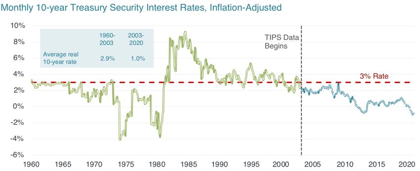
real equity returns like those in the stock market. However, climate change involves
intergenerational tradeoffs, raising difficult scientific, philosophical and legal questions
regarding equity across long periods of time. There is no scientific consensus about the
correct approach to discounting for the SCC.62

2010 IWG Approach and Progress: There are two possible approaches to discounting in
SCC calculations. First, a fixed discount rate can be used, as was implemented in the
IWG SCC calculations. The 2010 IWG used discount rates of 2.5 percent, 3 percent,
and 5 percent, while the Trump administration applied 3 percent and 7 percent, in
accordance with OMB Circular A-4. The 2010 IWG set the 3 percent discount rate as
the central case to be consistent with guidance from the OMB (2003) regarding the
interest rate on U.S. government bonds. This decision was also motivated by the
assumption that climate damages were projected to be uncorrelated with overall market
returns (eliminating the 7 percent rate, derived from equity markets) and thus used
insights from asset pricing theory that the riskless interest rate was appropriate.63

There have been profound changes in global capital markets since the publication of
Circular A-4 in 2003 that make it extraordinarily challenging to justify 3 percent as an
accurate estimate of the return on riskless investments. For example, the average ten-
year Treasury Inflation-Indexed Security (TIPS) rate over the available record of the
index (2003-present) is just 1.01 percent (see Figure 6).64 Similarly, recent research has
shown that the equilibrium real interest rate has declined substantially since the 1990s,
suggesting a lower discount rate is justified.65 Additionally, evidence from long-term real
estate investments suggests that for climate mitigation, which has payoffs over very long
periods of time, discount rates should be even lower than those used to discount costs
and benefits of shorter-lived investments.66 Overall, our judgement is that it is difficult
to defend a 3 percent discount rate for climate investments and there is now a
compelling case for a riskless discount rate of no higher than 2 percent.67

62 Gollier and Hammitt, “The Long-Run Discount Rate Controversy.”
63 Greenstone et al., “Developing A Social Cost of Carbon”
64 Board of Governors of the U.S. Federal Reserve System, “10-Year Treasury Inflation-Indexed Security.”
65 Bauer and Rudebusch, “Interest Rates Under Falling Stars.”
66 Giglio et al., “Climate Change and Long-run Discount Rates.”
67 A fixed rate below 2 percent does not contradict OMB Circular A-4 when a long-lived benefit stream is

under consideration: “If your rule will have important intergenerational benefits or costs you might
consider a further sensitivity analysis using a lower but positive discount rate in addition to calculating
net benefits using discount rates of 3 and 7 percent.” See OMB, “Circular A-4.”

 23

Figure 6: Monthly 10-year inflation-adjusted Treasury security interest rates. Figure shows monthly 10-
year Treasury security interest rates, adjusted for inflation, over the period 1960 to 2020. Nominal interest
rates, TIPS, and inflation data were retrieved from the Federal Reserve Bank of St. Louis. The Treasury
Inflation-Indexed Security (TIPS) rate is available starting in January 2003. Interest rates prior to 2003
are imputed by subtracting the annual inflation rate from the nominal interest rate.

There is also the possibility, however, that the riskless rate itself is not appropriate as
the central discount rate due to the unique risk properties of climate change and
uncertainty about future interest rates. Because discount rates reflect the returns to
investments that mitigate climate change, Americans are best served by using an
interest rate associated with investments that match the structure of payoffs from
climate mitigation. Capital asset pricing models recommend low discount rates in
scenarios where investments (in this case CO2 mitigation) pay off in “bad” states of the
world—that is, if climate damages are likely to coincide with a slowing overall economic
growth rate that for example could be due “tipping points” or large-scale human
responses to climate change, including mass migration.68 If on the other hand climate
damages act as tax on the economy (i.e., total damages are larger when the economy
grows faster), then higher discount rates like the average return in equity markets would
be merited.

68 Greenstone et al., “Developing A Social Cost of Carbon.”

 24

A second potential approach to deriving a discount rate is to explicitly account for
future economic growth using the so-called Ramsey equation,69 which is often referred to
as the prescriptive approach. This approach has been recommended by the NAS as a
“feasible and conceptually sound framework” (NAS, 2017). Rather than rely on observed
interest rates, it derives a discount rate from assumptions about three parameters: the
pure rate of time preference, the growth rate of consumption, and a parameter capturing
the decreasing marginal utility of consumption. Values for the first and third parameters
have been estimated in a large literature, while the consumption growth rate will depend
on the set of socioeconomic scenarios developed in the socioeconomic and emissions
module described above.70

The Ramsey approach has two key limitations. First, future economic growth is
uncertain, while the Ramsey equation is deterministic. Second, climate damages are
likely to be the highest in possible future scenarios where economic growth is the lowest.
Both facts imply that climate mitigation policies act as a form of insurance for the
future and imply a lower discount rate than is given by the Ramsey equation. Besides
these limitations, some find it unappealing that the Ramsey approach requires several
judgments by “experts” about the value of key parameters, rather than relying on
observed market interest rates.

Recommendation: We recommend continuing to rely on existing asset markets to guide
the choice of discount rates. Based on recent asset market trends, we recommend a
discount rate of no higher than 2 percent.

Ingredient 4: Global or Domestic Damages

Background and 2010 IWG Approach: Traditionally, regulatory cost-benefit analyses
(CBAs) have only considered the domestic benefits and costs of policies, on the theory
that what matters for U.S. policy are the effects of regulations on U.S. citizens.
However, unlike nearly every other environmental pollutant, CO2 emissions are

69 Ramsey, “A Mathematical Theory of Saving.”
70 The Ramsey equation expresses the discount rate as r = + η ⨉ g, where measures the pure rate of
time preference, g measures the growth rate of consumption, and η captures the decreasing marginal
utility of consumption. The consensus is that likely ranges between zero and two. Values for η have
been estimated in a large literature, and range from one to four, but are generally centered around two
(e.g., Arrow, 2007; Dasgupta, 2007, 2008; Hall, 2009; Weitzman, 2007, 2009).

 25

overwhelmingly a global problem. The damages caused by a ton of carbon emissions in
the United States are felt globally. Perhaps even more importantly, the United States is
harmed by emissions from abroad, so that when emissions are reduced in China, the
European Union, India, and elsewhere, Americans benefit. In light of the global nature
of the problem, and as a means to aid international negotiations in obtaining emissions
reduction commitments abroad, the IWG chose to use global damages to calculate the
SCC. In 2017, the Trump administration switched to only counting domestic damages in
the calculation of the SCC.

Progress: The overwhelming consensus amongst scientific and economic experts is that
the best policy is to include global damages.71 Although focusing exclusively on the
domestic costs of climate change may appear to put U.S. interests first, it does not;
indeed, a growing body of evidence demonstrates the opposite. Nearly 90 percent of
global emissions take place outside the United States, and since the climate does not
differentiate between a ton of carbon emitted in New York and a ton emitted in Beijing,
the United States will never be able to protect its citizens from climate change without
negotiating emissions reductions from other countries. If every nation uses a domestic
figure, all nations will lose; a global figure is necessary to overcome what might be seen
as a classic prisoner’s dilemma.72

Importantly, history shows us that when the United States accounts for the full global
cost of climate change it incentivizes other countries to reduce their own emissions,
which ultimately benefits the United States more than any purely domestic climate
policy could. As noted above, some nations simply borrowed the U.S. SCC. And in some
cases, the use of a global SCC, by the United States, plausibly contributed to
international action. For example, in 2014 the U.S. EPA proposed the Clean Power
Plan, and within four months the United States extracted a promise from China to
make significant reductions in its own emissions.73 Altogether, it is estimated that the
United States was able to leverage 6.1-6.8 tons of CO2 reductions from other countries
for every ton that it pledged to cut in the Paris Climate Agreement.74 The global
SCC—that is, an SCC informed by global damages, not just domestic—is an ingredient
in efforts to procure the necessary international action.

71 NAS, “Valuing Climate Damages.”
72 For relevant discussion, see Kotchen, “Which Social Cost of Carbon?”
73 Greenstone, “United States House Committee.”
74 Houser, “Calculating the Climate Reciprocity Ratio.”

 26