ValueNetQP: Learned one-step optimal control for legged locomotion
←
→
Page content transcription
If your browser does not render page correctly, please read the page content below
Proceedings of Machine Learning Research vol 144:1–12, 2022

                                          ValueNetQP: Learned one-step optimal control for legged locomotion

                                         Julian Viereck                                                                           JVIERECK @ NYU . EDU

                                         Avadesh Meduri                                                                             AM 9789@ NYU . EDU

                                         Ludovic Righetti                                                              LUDOVIC . RIGHETTI @ NYU . EDU
arXiv:2201.04090v1 [cs.RO] 11 Jan 2022

                                                                                                 Abstract
                                               Optimal control is a successful approach to generate motions for complex robots, in particular for
                                               legged locomotion. However, these techniques are often too slow to run in real time for model pre-
                                               dictive control or one needs to drastically simplify the dynamics model. In this work, we present a
                                               method to learn to predict the gradient and hessian of the problem value function, enabling fast reso-
                                               lution of the predictive control problem with a one-step quadratic program. In addition, our method
                                               is able to satisfy constraints like friction cones and unilateral constraints, which are important for
                                               high dynamics locomotion tasks. We demonstrate the capability of our method in simulation and
                                               on a real quadruped robot performing trotting and bounding motions.
                                               Keywords: Trajectory optimization, value function learning, model based method, quadruped
                                               robot

                                         1. Introduction
                                         Motion generation algorithms for legged robots can be broadly classified in two classes. On one
                                         side, there are optimal control methods Ponton et al. (2021); Shah et al. (2021); Carpentier and
                                         Mansard (2018); Mastalli et al. (2020); Winkler et al. (2018). These methods are very general and
                                         versatile but are computationally demanding to run in realtime, for model-predictive control (MPC),
                                         on a robot. Oftentimes, optimal trajectories are computed offline first before being executed on the
                                         robot. On the other side are policy learning techniques like reinforcement learning Lee et al. (2020);
                                         Peng et al. (2020); Rudin et al. (2021); Xie et al. (2020); Tan et al. (2018), which learn a control
                                         policy directly as a neural network. The policy is trained to optimize a long horizon reward. These
                                         methods are often sample inefficient, are prone to sim-to-real issues when transferring the simulated
                                         policy to the real robot and have a ”hard-coded” policy as a neural network with limited constraint
                                         satisfaction guarantees.
                                             To improve sample efficiency and solve times, model based optimal control algorithms have
                                         been used speed up policy learning. The Guided Policy Search algorithm Levine and Koltun (2013)
                                         uses an iterative linear quadratic regulator (iLQR) and optimizes trajectories together with a neural
                                         network policy till convergence. The work in Mordatch and Todorov (2014) also uses trajectory
                                         based optimization method and optimizes a neural network policy at the same time. However, these
                                         methods do not preserves all the information from the initial trajectory optimizer. In addition, there
                                         is no way to add constraints when running the policy.

                                         © 2022 J. Viereck, A. Meduri & L. Righetti.
VALUE N ET QP
Alternatively, learning a value function from iLQR has been explored. In Zhong et al. (2013)
the authors approximate the value function at the terminal step of a MPC problem using different
function approximators. In Lowrey et al. (2018) the authors learn the value function and use MPC
for control as well. The authors do not incorporate constraints when solving for the final control
and also are limited by the speed of the MPC solver.
The idea to use an optimization algorithm with future reward prediction is part of the paper
from Kalashnikov et al. (2018). There, the authors learn the Q function for a problem for visual
manipulation. The optimal action to use on the robot is found by maximizing samples from the Q
function given the current state. However, this method does not rely on a model of the dynamics.
Closer to our work, the authors in Parag et al. (2022) propose a method to predict the value func-
tion gradient and hessian using Sobolev learning. However, we were not able to get good learning
results using Sobolev learning for our quadruped locomotion experiments. They also used a MPC
approach with a longer horizon, which increases solve times but potentially improve robustness to
the quality of learned value function. While they demonstrate promising results on simulated low
dimensional problems, their method was not tested on systems with complexity comparable to a
legged robot nor was it tested on real hardware.
In this paper, we propose a method to learn the gradient and Hessian of a value function orig-
inally computed by an optimal control solver (iLQR). We then formulate a simple quadratic pro-
gram (QP) which efficiently uses these learned functions for one-step model predictive control at
high control rates. Our method enables to significantly decrease computation time while retaining
the ability to generate the complex locomotion movements. By using the QP we are also able to
enforce constraints on our solution like friction and unilateral contact force constraints, which is not
possible with policy learning methods or with the iLQR algorithm. With this approach, we gen-
erate different dynamic locomotion gaits on a real quadruped robot such as trotting and bounding.
We show that it is possible to robustly generate these dynamic motions, with a single step horizon,
affording computation of optimal controls at 500 Hz.
Specifically, the paper contributions are as follows: 1) We propose a stable method for learning
the value function gradient and Hessian information from iLQR, 2) we introduce our method for
computing control commands from value function gradients and Hessians taking constraints into
account, and 3) we demonstrate our method on two locomotion tasks on a real robot. In the fol-
lowing sections we explain in detail our method. After this we describe our experimental setup and
show results on the simulated and real robot. Finally, we conclude.
2. Method
The method proposed in this paper is as follow. First, we optimize motions from different starting
positions and with different properties (e.g. different desired velocity) using iLQR. Second, we use
the optimized trajectories together with the associated value function expansion to learn a mapping
between the current feature transformed state φ(xt ) to the value function gradient and hessian at the
next time step. Finally, at run time, our optimal control problem is reduced to the resolution of a
simple quadratic program (QP) which minimizes the learned value function for the state at the next
time step while including important constraints such as friction pyramids and unilateral constraints.
The rest of this section presents the details of the approach. First, we re-state the iLQR re-
cursions. Then we describe how control is optimized given a predicted value function using a QP.
Finally, we explain how the value function gradients are learned using a neural network.
2VALUE N ET QP
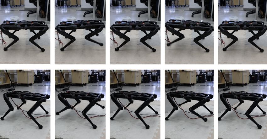
Figure 1: Time slices running the bounding (top) and trotting (bottom) motion on the real robot.
2.1. Optimal control with iLQR
We aim to solve an optimal control problem of the form
T
X
min lt (xt , ut ) (1)
u1 ,...,uT
t=1
s.t. xt+1 = ft (xt , ut )
where xt and ut are the system state and control vectors, lt an instantaneous cost, and ft describes
the system dynamics. The iLQR algorithm computes a local optimal control law starting from a
reference trajectory x̂. The method takes a second order expansion of the loss function lt and a first
order expansion of the dynamics ft around the reference trajectory. These approximations are used
to compute backward Riccati equations. The algorithm works in two passes.
In the backwards pass, the algorithm computes the second order approximation of the value
function V and Q function along the reference trajectory and proposes a control update δu. The
recursive update equations for the value function V and Q function are:
T
Qxt = ltx + ftx Vt+1
x
(2)
uT
Qut = ltu + ft Vt+1
x
(3)
xT
Qxx xx xx x x
t = lt + ft Vt+1 ft + Vt+1 f
xx
(4)
T
Qux
t = ltux + ftu Vt+1
xx x
ft + x
Vt+1 f ux (5)
T
Quu
t = ltuu + ftu Vt+1
xx u x
ft + Vt+1 f uu (6)
uu −1 u
Vtx = Qxt − Qxut (Qt ) Qt (7)
uu −1 ux
Vtxx = xx xu
Qt − Qt (Qt ) Qt , (8)
where ·xt , ·ut denotes the gradient at time t with respect to x and u and ·xx ux uu
t , ·t , ·t denotes the
Hessian terms with respect to xx, ux and uu at time t.
3VALUE N ET QP
In the forward pass, a line search is used to determine the best update αδu that would reduce
the trajectory cost when integrating the dynamics forward. To compute the control update δu, we
use the BoxDDP algorithm (Tassa et al. (2014)). This allows us to put bounds on the control and
e.g. avoid negative forces in the vertical direction.
2.2. Solving for control using a QP
From Bellman’s principle of optimally, it follows that to compute the optimal control ut and value
function at time t, it is sufficient to know the current cost and value function at time t + 1:
V (xt ) = min[lt (xt , ut ) + V (ft (xt , ut ))]. (9)
ut
Our goal is then to reduce the original optimal control problem to a one-step optimization problem
(as a QP) that will leverage a learned value function gradient and Hessian. We write this equation
as a constrained optimization problem:
V (xt ) = min [lt (xt , ut ) + V (xt+1 )]. (10)
ut ,xt+1
subject to xt+1 = ft (xt , ut )
Recall that in iLQR the value function is expressed along a nominal trajectory x̂t . We denote the
second order approximation for the value function as V (xt+1 ) ≈ Vt+1 0 + V x (x
t+1 t+1 − x̂t+1 ) +
1 T xx
2 (x t+1 − x̂ t+1 ) Vt+1 (x t+1 − x̂ t+1 ). Assuming a cost term of the form lt (xt , ut ) = lt (xt ) +
1 T uu
u
2 t t R ut we can solve for the arguments in the last minimization problem as follows:
1 T uu 0 x 1 T xx
argmin lt (xt ) + ut Rt ut + Vt+1 + Vt+1 (xt+1 − x̂t+1 ) + (xt+1 − x̂t+1 ) Vt+1 (xt+1 − x̂t+1 )
ut ,xt+1 2 2
subject to xt+1 = f (xt , ut )
which is equivalent to
x 1 T
argmin (Vt+1 − x̂Tt+1 Vt+1
xx
)xt+1 xx T uu
+ (xt+1 Vt+1 xt+1 + ut Rt ut ) , (11)
ut ,xt+1 2
subject to xt+1 = f (xt , ut )
where we removed constant terms and used the fact that Vt+1 xx is symmetric. Interestingly, our
problem only involves the gradient and Hessian of the value function and not its actual value. Also,
since our formulation contains a one step look up into the horizon it makes the nonlinear dynamics
f (x, u) linear. Subsequently, we can efficiently solve the above optimization problem with a QP to
obtain the optimal control ut .
2.3. Using the dynamics structure to reduce the QP
Since we work with system with a second dynamics, we can separate the state xt into the
order
position st and velocity vt part xt = st , vt . We then explicitly include the numerical inte-
gration scheme to simplify the previous QP. This will be important to facilitate learning. Start-
xx corresponding to s and v as V xx =
ing from eq. (11), writing the block components of Vt+1 t t t+1
4VALUE N ET QP
ss sv
s
Vt+1 Vt+1 x T xx Vt+1
vs
Vt+1 vv and (Vt+1 − x̂t+1 Vt+1 ) = V v
Vt+1
we get
t+1
" T T ss !#
s sv
Vt+1 st+1 1 st+1 Vt+1 Vt+1 st+1
argmin v + vs vv + uTt Rtuu ut , (12)
ut ,vt+1 Vt+1 vt+1 2 vt+1 Vt+1 Vt+1 vt+1
st+1 st + ∆t vt
subject to =
vt+1 vt + B u ut + B 0
where we rewrote the constraints on the dynamics using an Euler integration scheme st+1 = st +
∆t vt and linearization of the velocity dynamics B u and offset B 0 . Because st+1 is constrained
by st and vt , which are not part of the optimization variables, st+1 can be replaced in the last
optimization with st + ∆t vt . Applying this substitution and simplifying terms yields:
1
u∗t , vt+1
∗ v sv vv T uu
= argmin (Vt+1 + st+1 Vt+1 )vt+1 + vt+1 Vt+1 vt+1 + ut Rt ut . (13)
ut ,vt+1 2
subject to vt+1 = vt + B u ut + B 0
This formulation of the problem has multiple important benefits. First, the dimension of the op-
v +x
timization problem is smaller. In addition, the vector (Vt+1 sv vv
t+1 Vt+1 ) and the matrix Vt+1 are
smaller compared to equivalent entities written in the original problem. This size reduction will be
very important to yield good results once we learn these quantities using a neural network. Finally,
it will be easy to add state and control constraints to this QP, as we will show in the subsequent
sections.
2.4. Learning the value function gradient and Hessian
Given optimized iLQR trajectories, we can also recover the value function gradient and Hessian
at each time steps (cf. recursions of Sec. 2.1). We aim to predict the value function gradient
gt+1 = (Vt+1v +s sv vv
t+1 Vt+1 ) and Hessian Vt+1 . We do this by regressing the gradient and Hessian
directly to a feature transformed input state φ(xt ) (we will give an example of a feature transfor-
mation of the input state in the experimental section below). The regression is solved under a L1
loss using gradient descent and a neural network. We call the neural network the value function
network (ValueNet). As for the network output, we flatten the Hessian matrix Vt+1 vv into a vector
and concatenate it with the gradient g into a single target vector for the regression task. To use the
vv in the QP we must ensure that the matrix is positive definite. We do this as follows:
Hessian Vt+1 T
First, we make sure the matrix is symmetric by instead computing 1/2 Vt+1 vv + V vv
t+1 . Then, we
compute the eigenvalue and eigenvector of the matrix and set negative eigenvalues to small positive
eigenvalues. We found in our experimental results that this regularization worked well.
In all our experiments, we use the same neural network architecture. We use a 3 layer fully
connected feedforward neural network with 256 neurons per layer. As activation function we use
tanh. The network is trained for 256 epochs with a batch size of 128 using Adam and a learning
rate of 3e-4. During our experiments we noticed that small changes in the predicted gradient and
Hessian lead to drastic different results when solving the QP. To mediate this problem, we found it
useful to normalize the gradient and hessian prediction to zero mean and unit variance.
5VALUE N ET QP
3. Experimental setup
In the following, we describe our experimental setup and experiments. We demonstrate our method
on two kinds of locomotion tasks: bounding and trotting on a simulated and real quadruped robot,
where the desired velocity can be controlled and the robot can handle push perturbations. In our
experiments we use the Solo12 quadruped from the Open Dynamic Robot Initiative (Grimminger
et al. (2020)). The 12 joints are torque controlled, making it an ideal platform to test model predic-
tive control methods. In all experiments, we use a Vicon motion capture system and IMU to get an
estimate of the robot base position and velocity.
3.1. Dynamics model
To illustrate the capabilities of our approach, we use a standard, simplified centroidal dynamics
model of a quadruped. We model the state xt as xt = [ct , αt , ċt , ω] where ct is the position of the
center of mass (CoM), αt is the orientation of the base and ċt , ω are the respective velocities. All
quantities are expressed in an inertial (world) frame. The control inputs are the forces applied by
the feet of the quadruped Fi , where Fi denotes the contact force at the i-th leg and ri the position of
the i-th leg contact location. The discretized dynamics equations are then
ċt
ct+1 ct
P Fωi t
αt+1 αt
ċt+1 = ċt + ∆t
, (14)
i m − G
P Fi ×(ri −ct )
ωt+1 ωt i I
where G = [0, 0, 9.81]T m/s2 is the gravity vector and m = 2.5 kg is the robot mass. I denotes
the rotational inertia mass matrix of the base joint. Since the inertia mass matrix does not change
significantly for trotting and bounding, we keep it constant throughout all of our experiments. Note
however that the associated optimal control problem is not convex due to the cross product.
3.2. Pattern generator
To generate example bounding and trotting motions, we need to know the desired foot locations ri .
For this, we utilize a pattern generator. Given an initial CoM position and velocity, desired CoM
velocity and information about the gait (i.e. the sequence of endeffector contacts with the ground) ,
the pattern generator generates the foot locations ri .
When the foot i goes into contact, the foot location is computed using the following Raibert-
inspired heuristic Raibert et al. (1984)
tstance
ri = ct + shoulderi + ċ + kraibert (vcmd − ċ), (15)
2
where shoulderi is the offset of the endeffector in the neutral position from the CoM, tstance is
stance phase duration, kraibert is a constant (we choose 0.03 in all our experiments) and vcmd is
the commanded / desired velocity of the CoM. To evaluate this equation, we interpolate between
the current CoM velocity ċ and the desired velocity. In particular, at each timestep we update the
planned CoM velocity as
ċ = (1 − vα ) ċ + vα vcmd , (16)
where we choose vα as 0.02 in all our experiments. Using this control, the robot will bring the base
velocity slowly towards the desired velocity.
6VALUE N ET QP
3.3. iLQR data generation and network training
To train our ValueNet we use samples from iLQR optimized trajectories. We generate many iLQR
trajectories by putting the robot into a random initial state (random initial position and velocity),
sample a desired velocity command in a random direction (up to 0.6 m/s) and generate the feet
locations ri using the pattern generator. As iLQR cost l(xt , ut ) in eq. (1) we use a quadratic cost
between the current state xt and desired state x̂t where there is no weight for the horizontal position.
x , v y , 0, . . . , 0]. In addition, we use a quadratic cost to
The desired state is x̂ = [0, 0, 0.21, vcmd cmd
regularize the control.
Given that we optimize a finite horizon problem, we know that the value function gradient and
Hessian will be very different from their stationary values for the infinite horizon problem towards
the end of the horizon. This change in magnitude makes learning to predict the value function
gradient and Hessian difficult if value function information at the end of the optimized trajectory
was used. To overcome this problem, we optimize many small iLQR trajectories and use only the
information from the first timestep. We do this as follows: We first optimize a longer (four gait
cycles long) horizon trajectory from a random initial configuration using iLQR. Then, for each of
the timesteps belonging to the first 1.5 cycles along this trajectory, we initialize a shorter iLQR
trajectory (2.5 gait cycles long). These shorter iLQR trajectories are warm started using the longer
iLQR trajectories and optimized. We then store the information from the first time step in form
of φ(x0 ) as well as value function gradient and Hessian. For the trotting and bounding motion
we optimize 2048 long iLQR trajectories leading to around 313000 training samples. As time
discretization we use ∆t = 0.004 s.
As discussed before, we perform a feature transformation φ(xt ) on our states before using them
as input to the neural network. It is important that the network does not overfit to the current absolute
position of the robot in the horizontal plane. Therefore, φ(xt ) is using the full state xt besides the
CoM position in horizontal plane. Besides this reduced state, we found it beneficial to include also
the relative positions of the endeffectors with respect to the CoM in φ(xt ). We also incorporate
information whether an endeffector is in contact with the ground at a given state. We do this by
encoding the active/inactive contact state as {0, 1} respectively and pass four numbers (one for each
leg) as input. Lastly, we also pass the desired velocity vcmd and the contact time of each leg as input.
The contact time is the time until the foot either is about to leave contact or how long it is still in
contact (depending on the current contact configuration).
3.4. Integration of QP in Whole body control
At each control cycle, forces Fi are computed by specializing the QP in eq. (13) with the dynamic
models from eq. (14), adding important contact constraints and the learned ValueNet:
∗ ∗ 1 vv 1 T FF
Ft , vt+1 = argmin gt+1 vt+1 + vt+1 Vt+1 vt+1 + Ft Rt Ft . (17)
Ft ,vt+1 2 2
vt+1 = vt + B F Ft + B 0
|Fx | ≤ µFz
subject to
|Fy | ≤ µFz
0 ≤ Fz ≤ 30,
where we added friction pyramid constraints. We use a friction coefficient of µ = 0.6 in our
experiments. We also impose unilateral contact forces and limit the z-force to 30 N m for safety
7VALUE N ET QP
Simulation
0.75
Robot base x-velocity
0.50 Commanded x-velocity
0.25
Speed [m/s]
0.00
0.25
0.50
0.75
0 2 4 6 8
Real robot
0.50
0.25
Speed [m/s]
0.00
0.25
0.50
0.75
0 2 4 6 8 10
Time [s]
Figure 2: Velocity tracking on the simulated (top) and real robot (bottom) for a bounding motion.
Simulation
0.75 Robot base x-velocity
0.50 Commanded x-velocity
0.25
Speed [m/s]
0.00
0.25
0.50
0.75
0 2 4 6 8
Real robot
0.75
0.50
0.25
Speed [m/s]
0.00
0.25
0.50
0 2 4 6 8 10
Time [s]
Figure 3: Velocity tracking on the simulated (top) and real robot (bottom) for a trotting motion.
reason (roughly double of what is usually applied). If not stated otherwise, the final controller runs
at 500 Hz.
We use a whole-body controller to map these commands to actuation torques. First, we must
generate motions for the endeffector to reach the desired location ri . Using eq. (15) we compute the
desired location of the swing-feet and plan a fifth order polynominal trajectory for the x/y direction
and 3rd order polynominal for the z direction in Cartesian space for the endeffector motions. We
track the desired endeffector position êi and velocity ê˙ i using the following impedance controller
X n o
τ= T
Jc,i P (êi − ei ) + D(ê˙ i − ėi ) + Fi , (18)
i
where τ is vector of actuation torques, Jc,i is the contact Jacobian for leg i, P and D are gains and ei
is the position of the endeffector. It is important, however, to keep in mind that the most important
part of the locomotion behavior, including proper balancing and CoM motion, is generated by the
one-step QP solver.
8VALUE N ET QP
Simulation Real robot
20 Fx
Fy
Fz
15
Force [N]
10
5
0
0.0 0.2 0.4 0.6 0.8 1.0 0.0 0.2 0.4 0.6 0.8 1.0
Time [s] Time [s]
Figure 4: Force profile of the first second from tracking the bounding motion in fig. 2. The left plot
shows the results from simulation and the right plot shows results from the real robot.
4. Experiments and results
Using the method and experimental setup described above, we perform a set of experiments in
simulation and on the real hardware. The experiments are designed to demonstrate that our proposed
method works and can be robustly applied on a real robot. Examples of the motions can be found
in fig. 1 and in the accompanying video 1 .
4.1. Velocity tracking
We evaluate the ability of our method to track a desired velocity, using the bounding and trotting
motion on the simulated and real robot. We let the robot bound/trot forward and backwards for a few
seconds at different commanded velocities. The results are shown in fig. 2 and fig. 3. We observe
that the velocity is tracked very well both in simulation and on the real robot, while the exact same
controller and learned value function are used. It is interesting to see that the one-step QP is able to
generate a diverse set of stable motions thanks to the learned value function.
4.2. Robustness to external disturbances
To test robustness of our proposed method, we perform two sets of experiments on the real robot:
First, we manually push the robot while keeping it in place. In the second experiment, we place
obstacles with 2.5 cm height in the path of travel and let the robot run across these obstacles.
We repeat both experiments for the trotting and bounding motion. The results are shown in the
accompanying video. As one can see in the video, our method is able to keep the robot stable when
moving over the obstacles and is robust to random pushes.
4.3. Smoothness of control profile
Recall that our method is computing desired forces at the endeffectors as control output. Especially
when working on the real hardware it is important that the computed forces (and thereby the com-
puted torques using eq. (18)) are smooth enough to prevent the robot from shaking and destabilizing.
In fig. 4, we show the force profile generated by our method on the bounding task shown in fig. 2
for the first second.
1. Video of the experimental results https://youtu.be/qcBwlyZjnRA
9VALUE N ET QP
As one can see from the plot, the force profile is quite smooth in simulation. On the real robot,
the forces are a bit more noisy but this is expected given noisy measurements from the real robot
that are fedback in the QP (our simulation is noise free). Still, the forces on the real system are
smooth enough and not destabilize the bounding or trotting motion.
4.4. Necessity for QP constraints
One of the benefits of our method is that we are able to add constraints when solving for the control
in eq. (13). We verify the necessity for the bounds by disabling them for the trotting and bounding
motion. When we disable the QP bounds for the trotting motion, we see negative Fz forces being
applied. Still, the motion of the robot stays robust. In contrast, when disabling the QP bounds on the
bounding motion, the legs start slipping and the robot motion becomes unstable. This demonstrates
the necessity of the QP bounds and the benefit of having these constraints.
4.5. Reducing value function gradient and hessian prediction frequency
By default we are evaluating the neural network to get a new value function gradient and Hessian
at each control step at 500 Hz. In this experiment we study the prediction frequency has on the
stability of the motion on the robot. To do this, we reduce the update frequency of the predicted
gradient and Hessian while running the rest of the controller (evaluating the QP and impedance
controller) at 500 Hz. When running the bounding motion, we are able to reduce the value function
prediction from 500 Hz to 62.5 Hz before the robot becomes unstable (shown in the accompanying
video). This is an interesting observation, as it shows that it is not necessary to evaluate the value
function at the same rate as the controller, therefore reducing computation.
5. Conclusion and future work
In this paper, we presented a method to reduce a (non-convex) optimal control problem into a
one-step QP by learning the value function gradients and Hessians computed on the original prob-
lem. We demonstrated the approach on trotting and bounding motions with velocity control and
showed that the method could be directly used on a real quadruped robot. This approach enables to
significantly reduce computational complexity, enabling model predictive control to generate non-
trivial locomotion behaviors. We demonstrated and analyzed the robustness and capabilities of this
method in simulation and on a real quadruped robot. As future work we are planning to study how
the learned value function gradient and Hessian information can be used as terminal costs for longer
horizon model predictive control. In addition, we intend to apply the method on a biped robot,
which is more unstable and a humanoid robot with more degrees of freedom.
Acknowledgments
This work was supported by New York University, the European Union’s Horizon 2020 research
and innovation program (grant agreement 780684) and the National Science Foundation (grants
1825993, 1932187, 1925079 and 2026479).
10VALUE N ET QP
References
Justin Carpentier and Nicolas Mansard. Multicontact locomotion of legged robots. IEEE Transac-
tions on Robotics, 34(6):1441–1460, 2018.
Felix Grimminger, Avadesh Meduri, Majid Khadiv, Julian Viereck, Manuel Wüthrich, Maximi-
lien Naveau, Vincent Berenz, Steve Heim, Felix Widmaier, Thomas Flayols, et al. An open
torque-controlled modular robot architecture for legged locomotion research. IEEE Robotics and
Automation Letters, 5(2):3650–3657, 2020.
Dmitry Kalashnikov, Alex Irpan, Peter Pastor, Julian Ibarz, Alexander Herzog, Eric Jang, Deirdre
Quillen, Ethan Holly, Mrinal Kalakrishnan, Vincent Vanhoucke, et al. Qt-opt: Scalable deep
reinforcement learning for vision-based robotic manipulation. arXiv preprint arXiv:1806.10293,
2018.
Joonho Lee, Jemin Hwangbo, Lorenz Wellhausen, Vladlen Koltun, and Marco Hutter. Learning
quadrupedal locomotion over challenging terrain. Science robotics, 5(47), 2020.
Sergey Levine and Vladlen Koltun. Guided policy search. In International conference on machine
learning, pages 1–9. PMLR, 2013.
Kendall Lowrey, Aravind Rajeswaran, Sham Kakade, Emanuel Todorov, and Igor Mordatch. Plan
online, learn offline: Efficient learning and exploration via model-based control. arXiv preprint
arXiv:1811.01848, 2018.
Carlos Mastalli, Rohan Budhiraja, Wolfgang Merkt, Guilhem Saurel, Bilal Hammoud, Maximilien
Naveau, Justin Carpentier, Ludovic Righetti, Sethu Vijayakumar, and Nicolas Mansard. Crocod-
dyl: An efficient and versatile framework for multi-contact optimal control. In 2020 IEEE Inter-
national Conference on Robotics and Automation (ICRA), pages 2536–2542. IEEE, 2020.
Igor Mordatch and Emo Todorov. Combining the benefits of function approximation and trajectory
optimization. In Robotics: Science and Systems, volume 4, 2014.
Amit Parag, Sébastien Kleff, Léo Saci, Nicolas Mansard, and Olivier Stasse. Value learning from
trajectory optimization and sobolev descent: A step toward reinforcement learning with superlin-
ear convergence properties. In International Conference on Robotics and Automation, 2022.
Xue Bin Peng, Erwin Coumans, Tingnan Zhang, Tsang-Wei Lee, Jie Tan, and Sergey Levine. Learn-
ing agile robotic locomotion skills by imitating animals. arXiv preprint arXiv:2004.00784, 2020.
Brahayam Ponton, Majid Khadiv, Avadesh Meduri, and Ludovic Righetti. Efficient multicontact
pattern generation with sequential convex approximations of the centroidal dynamics. IEEE
Transactions on Robotics, 2021.
Marc H Raibert, H Benjamin Brown Jr, and Michael Chepponis. Experiments in balance with a 3d
one-legged hopping machine. The International Journal of Robotics Research, 3(2):75–92, 1984.
Nikita Rudin, David Hoeller, Philipp Reist, and Marco Hutter. Learning to walk in minutes using
massively parallel deep reinforcement learning. arXiv preprint arXiv:2109.11978, 2021.
11VALUE N ET QP
Paarth Shah, Avadesh Meduri, Wolfgang Merkt, Majid Khadiv, Ioannis Havoutis, and Ludovic
Righetti. Rapid convex optimization of centroidal dynamics using block coordinate descent.
arXiv preprint arXiv:2108.01797, 2021.
Jie Tan, Tingnan Zhang, Erwin Coumans, Atil Iscen, Yunfei Bai, Danijar Hafner, Steven Bohez,
and Vincent Vanhoucke. Sim-to-real: Learning agile locomotion for quadruped robots. arXiv
preprint arXiv:1804.10332, 2018.
Yuval Tassa, Nicolas Mansard, and Emo Todorov. Control-limited differential dynamic program-
ming. In 2014 IEEE International Conference on Robotics and Automation (ICRA), pages 1168–
1175. IEEE, 2014.
Alexander W Winkler, C Dario Bellicoso, Marco Hutter, and Jonas Buchli. Gait and trajectory opti-
mization for legged systems through phase-based end-effector parameterization. IEEE Robotics
and Automation Letters, 3(3):1560–1567, 2018.
Zhaoming Xie, Patrick Clary, Jeremy Dao, Pedro Morais, Jonanthan Hurst, and Michiel Panne.
Learning locomotion skills for cassie: Iterative design and sim-to-real. In Conference on Robot
Learning, pages 317–329. PMLR, 2020.
Mingyuan Zhong, Mikala Johnson, Yuval Tassa, Tom Erez, and Emanuel Todorov. Value function
approximation and model predictive control. In 2013 IEEE symposium on adaptive dynamic
programming and reinforcement learning (ADPRL), pages 100–107. IEEE, 2013.
12You can also read